How Electromagnetism & Quantum Mechanics Work & Where Physics Went Wrong

This post includes the video, transcript, and slides for my Keynote Address to the IEEE EMC & SIPI Symposium August 5, 2026: “How Electromagnetism & Quantum Mechanics Work & Where Physics Went Wrong.” Thanks again to Benoit Derat and the Symposium organizers for the opportunity to join their distinguished line up of speakers.

Abstract:

This talk presents the central thesis of the Fields & Energy Project: electromagnetism is not best understood as the action of a single entity, the photon, endowed with the mutually contradictory properties of localized particle and non-localized wave. Instead, electromagnetic phenomena emerge from the interaction of two distinct elements: spatially extended fields that behave as waves, and energy that, in the quantum limit, is transferred in discrete amounts. Fields guide energy.

Through examples drawn from fields and their interactions, antenna theory, and atomic emission and absorption, this talk demonstrates how the fields-and-energy model provides a conceptually coherent and technically productive framework. This perspective clarifies long-standing puzzles associated with radiation reaction and wave-particle duality and connects Maxwellian theory, quantum emission and absorption, and engineering practice within a unified narrative.

The broader aim is to recover conceptual clarity in the foundations of physics, to reestablish continuity between classical and quantum descriptions, and to examine the historical and philosophical developments that shaped modern interpretations. By restoring a disciplined distinction between fields and energy, the talk argues for a simpler and more intelligible account of electromagnetic processes — one capable of unifying principles across physics and engineering.

Transcript

This is a machine-generate transcription of the audio track, lightly edited.

Introduction by Benoit Derat, Technical Program Chair

Benoit: I won’t read Hans’s biography, you can find it also in the program, you can find it on the slide and you can read it by yourself. Instead of that, I will tell you a more personal story.

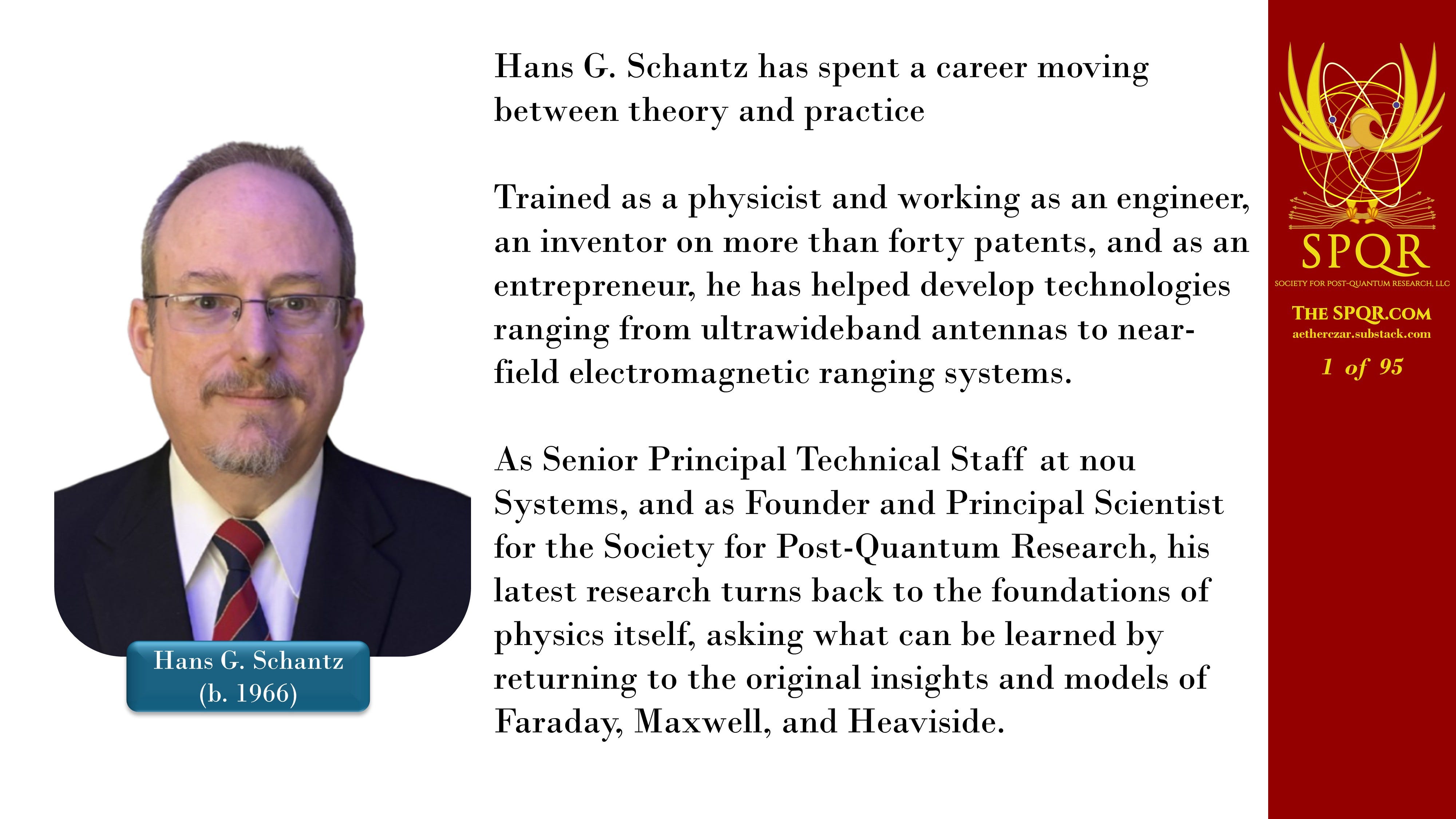
So when I was a PhD student, the first conference I attended. I’m sorry to say that was not the IEEE-EMC symposium. That was back in 2005, the IEEE AP Symposium in Washington DC back then. And I found on one of the technical sessions a presentation with an intriguing name and so I decided to enter the room and see what was presented there.

That was my first contact with Dr. Hans Schantz where I saw him giving a complete different take at how dipole radiation in time domain, how the energy transfers. I was literally blown away by the way he was looking at things. And he was at this time finishing a book, The Art and Science of Ultrawideband Antennas.

Second Edition, 2015.

And as a consequence, I decided to buy it. And after reading that book, I would say, Dr. Schantz’s research had his hook on me. So, I kept on following his work over the years, and as I was appointed Technical Program Chair, I was delighted to have a possibility to offer you a talk from Hans today, who will present you how electromagnetism and quantum mechanics work and where physics went wrong.

I think it’s gonna be a thought-provoking presentation. I’m looking forward to also have a Q&A with this audience. Hans, welcome on stage. Please welcome the speaker.

Introduction by Hans G. Schantz, Keynote Speaker

Hans: Thank you, Benoit. Well, I’d like to thank Benoit and the Technical Program Committee for this wonderful opportunity to be with you here today. My topic is going to be “how electromagnetism and quantum mechanics work and where physics went wrong.”

An Introduction About Models

I want to begin by talking a little bit about the concept of a model.

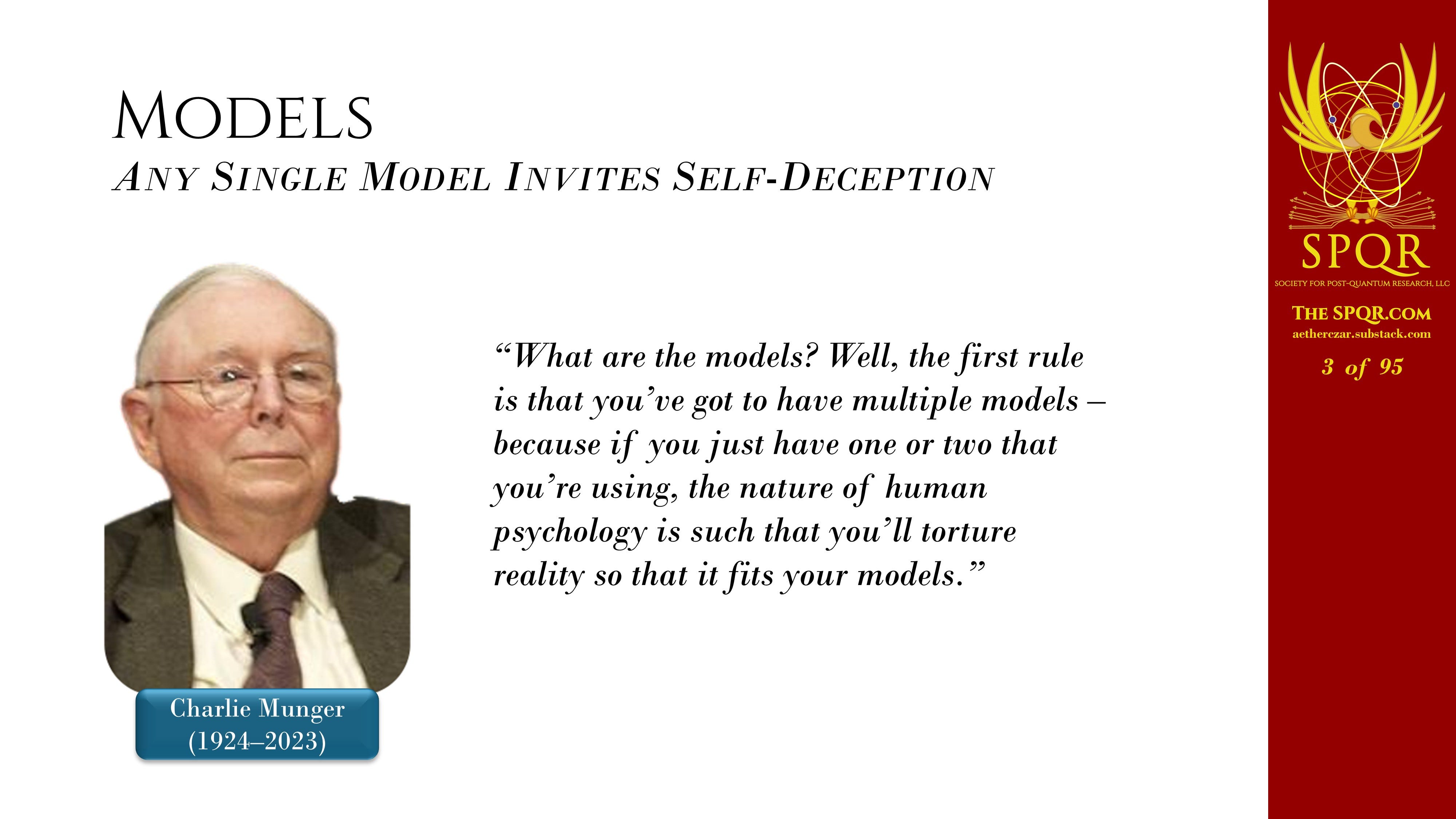
Charlie Munger, who is Warren Buffet’s, one of his financial advisors and partners, commented that if you only have one or two models, human psychology being what it is, you will distort reality to fit your model.

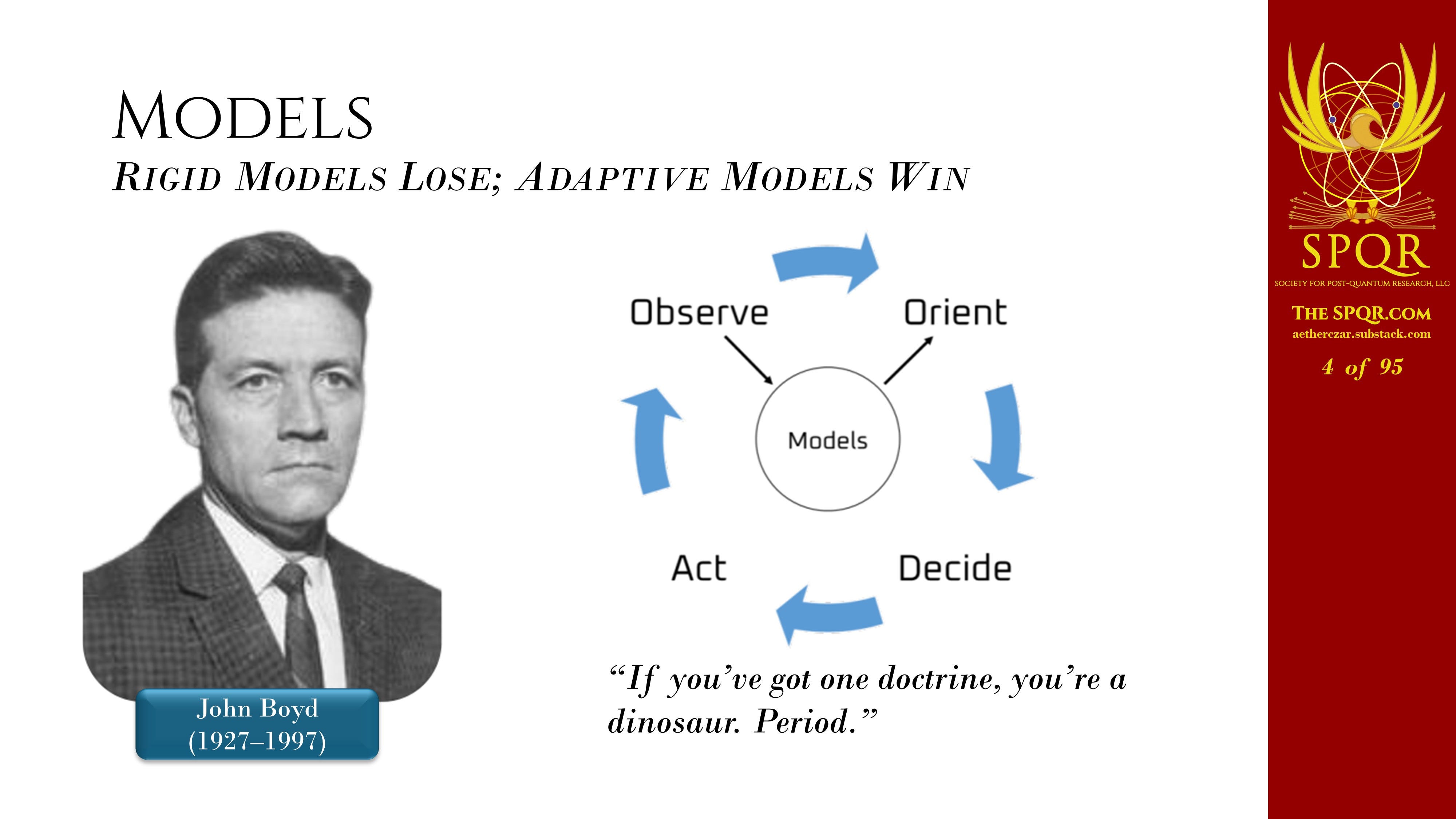
The famous warfighter John Boyd came up with the concept of the OODA loop, observe, orient, decide, and act. You observe what’s going on in your tactical situation. You use your models, or as he called them, doctrines, to organize that information and orient yourself to try to control the pace of your tactical activities. His comment, if you’ve only got one doctrine, you’re a dinosaur, period.

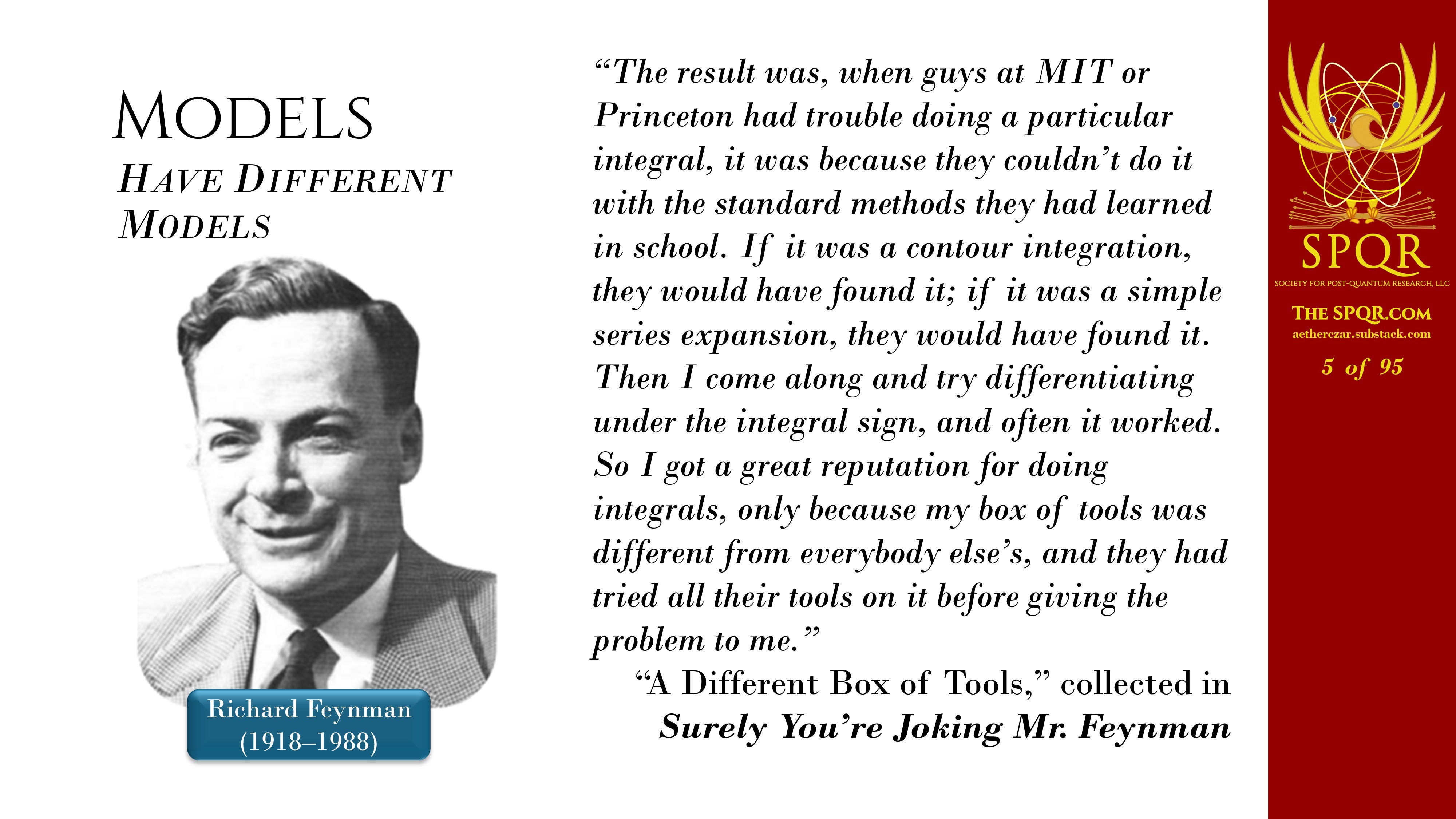
And from the context of physics and science, Richard Feynman noted in Surely You’re Joking, Mr. Feynman, that he had stumbled across a unique method for solving some difficult integrals, differentiating under the It was a technique that was not widely known or applied and the result was that his colleagues and fellow students would bring problems to him and he would be able to solve it because he had, as he called it, a different box of tools, a useful model that was not in common use.

That brings me to the question of models in electromagnetism.

Having a rich repertoire of models is essential to the practicing engineer, providing multiple ways to look at and solve and interpret and understand problems. Today I’m going to be sharing with you a model I call the “Fields & Energy” model. I’m going to talk about fundamentals and origins of electromagnetism, where physics went wrong, and finally how electromagnetism and quantum mechanics work.

Fundamentals and Origins

We can start by looking at what Faraday accomplished. He would heat a sheet of wax paper and sprinkle iron filings on it and put it on top of a magnet, allow it to cool, capture the patterns and study these mysterious field lines.

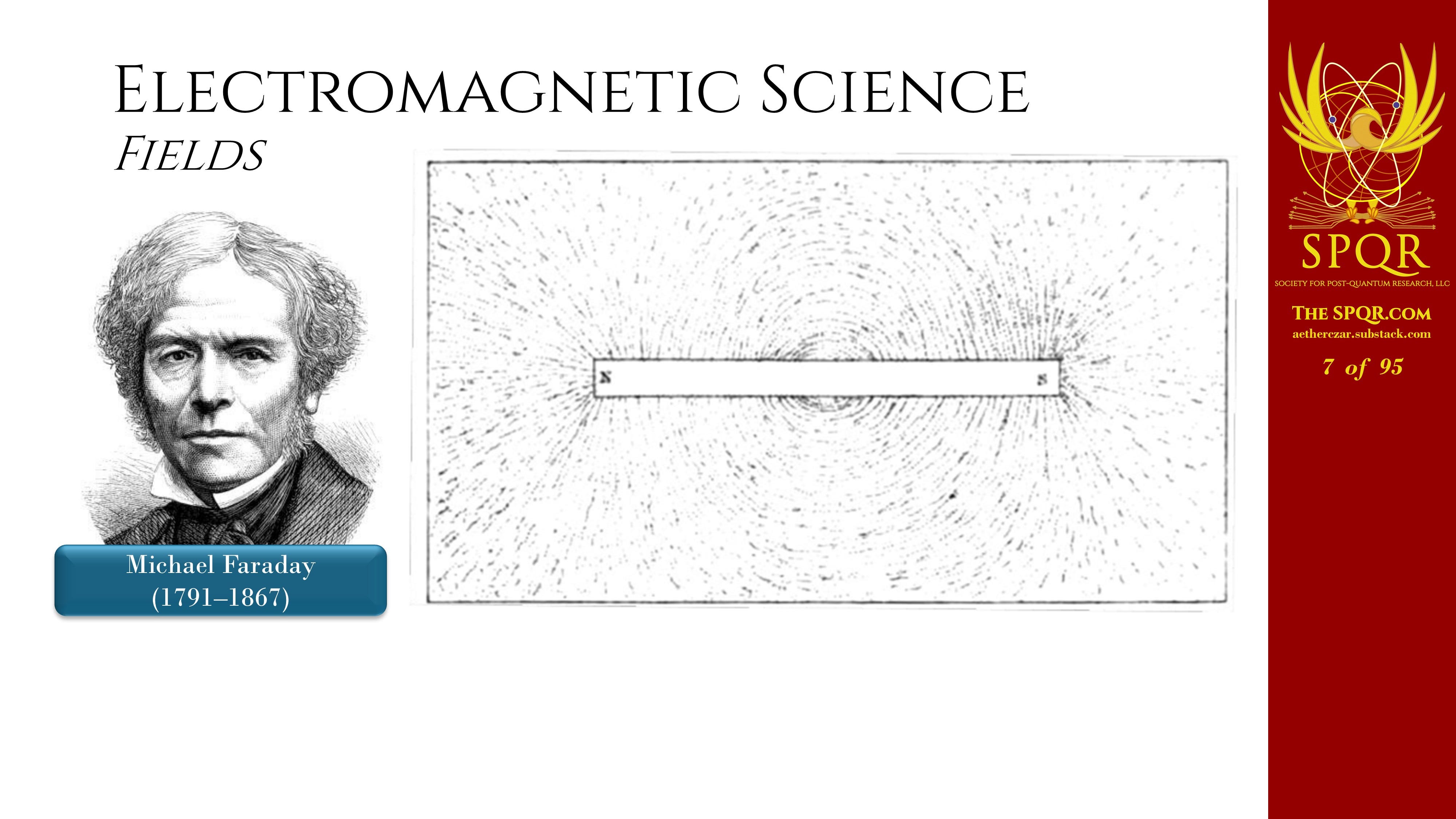
That gave him the insight to develop the laws of induction and the fundamental physics behind all the motors and generators that we use today.

Those insights were put into a mathematical form by James Clerk Maxwell.

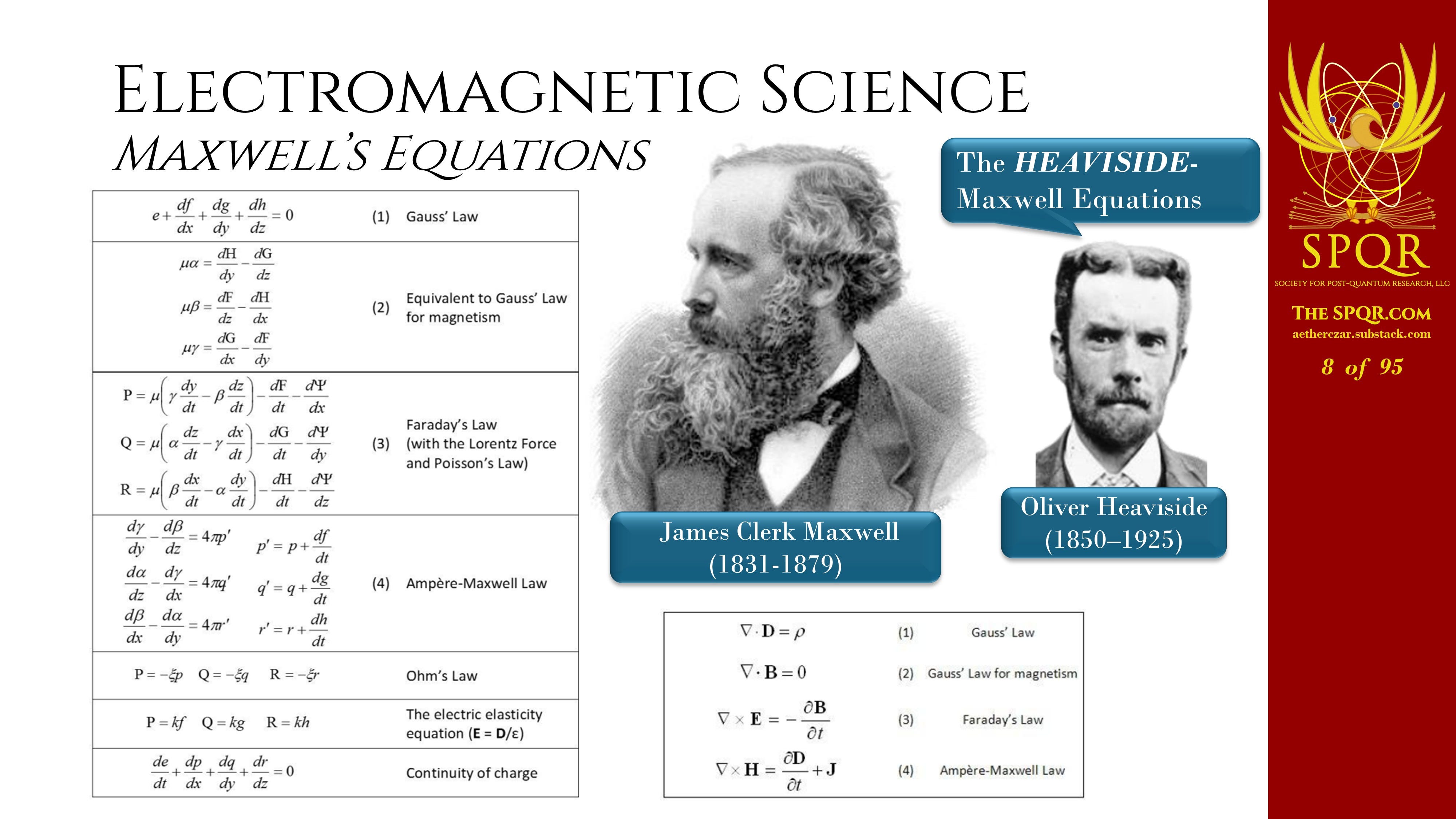
Now, those, of course, were streamlined by Oliver Heaviside into the four familiar vector relationships that we use today. And what he discovered is that an electromagnetic wave was an electric wave and a magnetic wave operating at right angles.

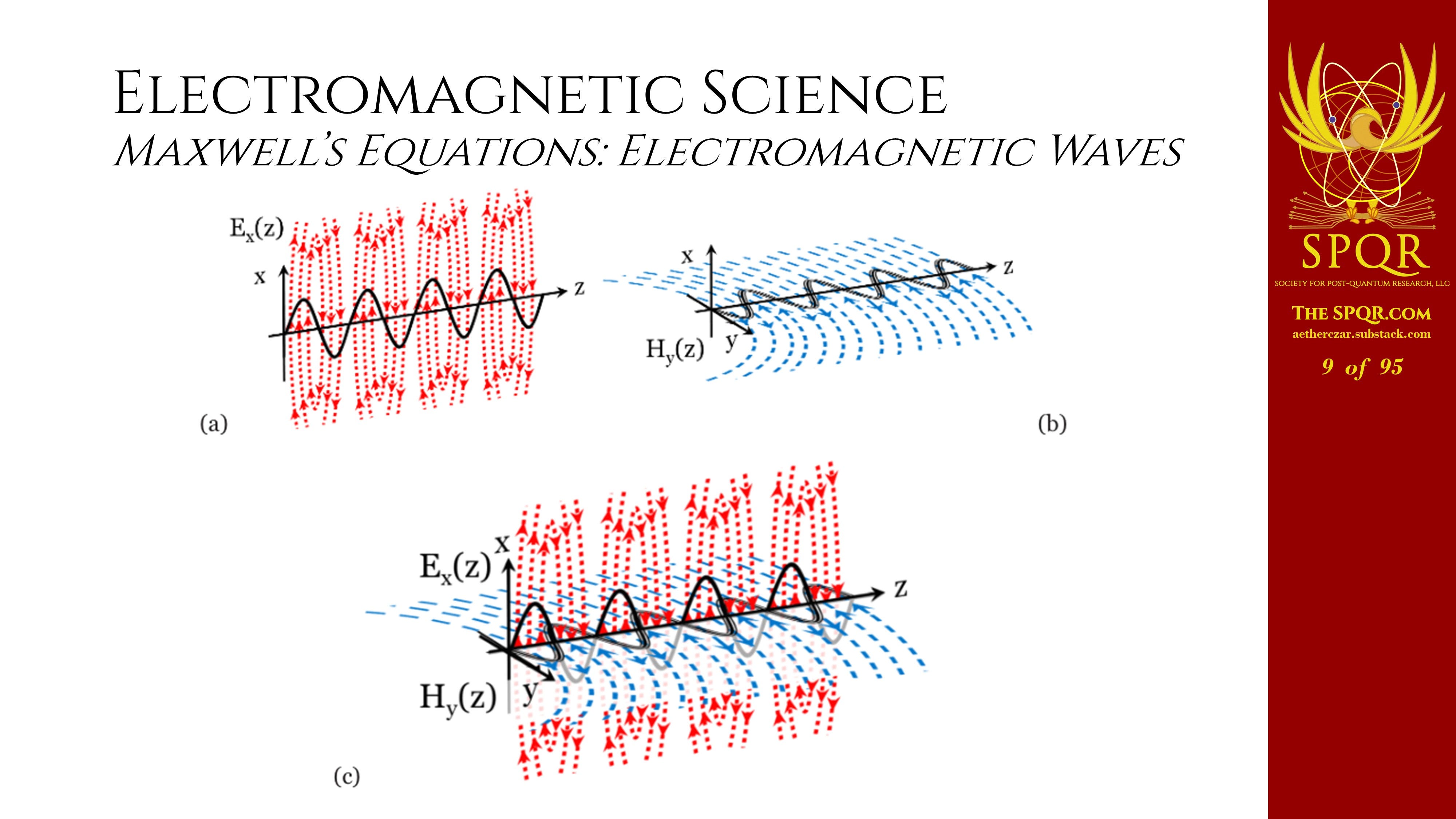
And he demonstrated that they move at the speed of light, suggesting that light was an electromagnetic phenomenon.

Telegraphy & The Origins of Applied Electromagnetism

The first transatlantic telegraph cable was laid in 1858 and it very quickly failed. It never worked very well because the signals were muddied and distorted. And it was because of poor design and poor understanding of the fundamental underlying science.

The Victorian Internet: The Remarkable Story of the Telegraph and the Nineteenth Century’s On-line Pioneers by Tom Standage captures the excitement of the social revolution unleashed by telegrapy.

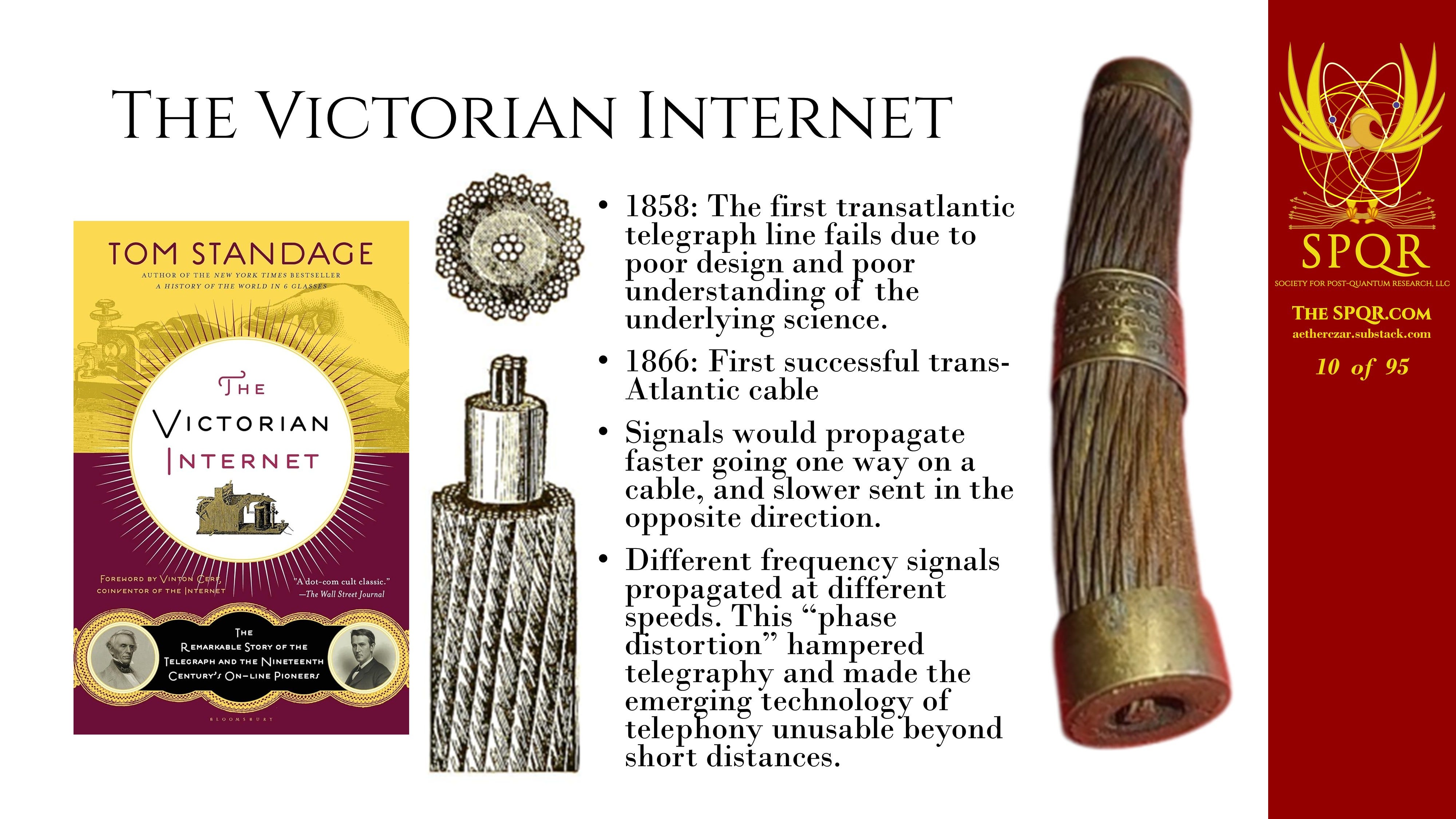
It was 1866 before the first successful cable was laid. Some of the anomalies that were seen were things like signals propagating faster in one direction than in the other direction. And, of course, the frequency dispersion completely limited the ability to send signals very long distances at any reasonable rate and put a practical limitation on being able to do telephony at any distance beyond very, very short ranges.

Those problems were solved by this guy, Oliver Heaviside. He came up with the telegrapher’s equation to describe how the transmission lines that we still deal with today work.

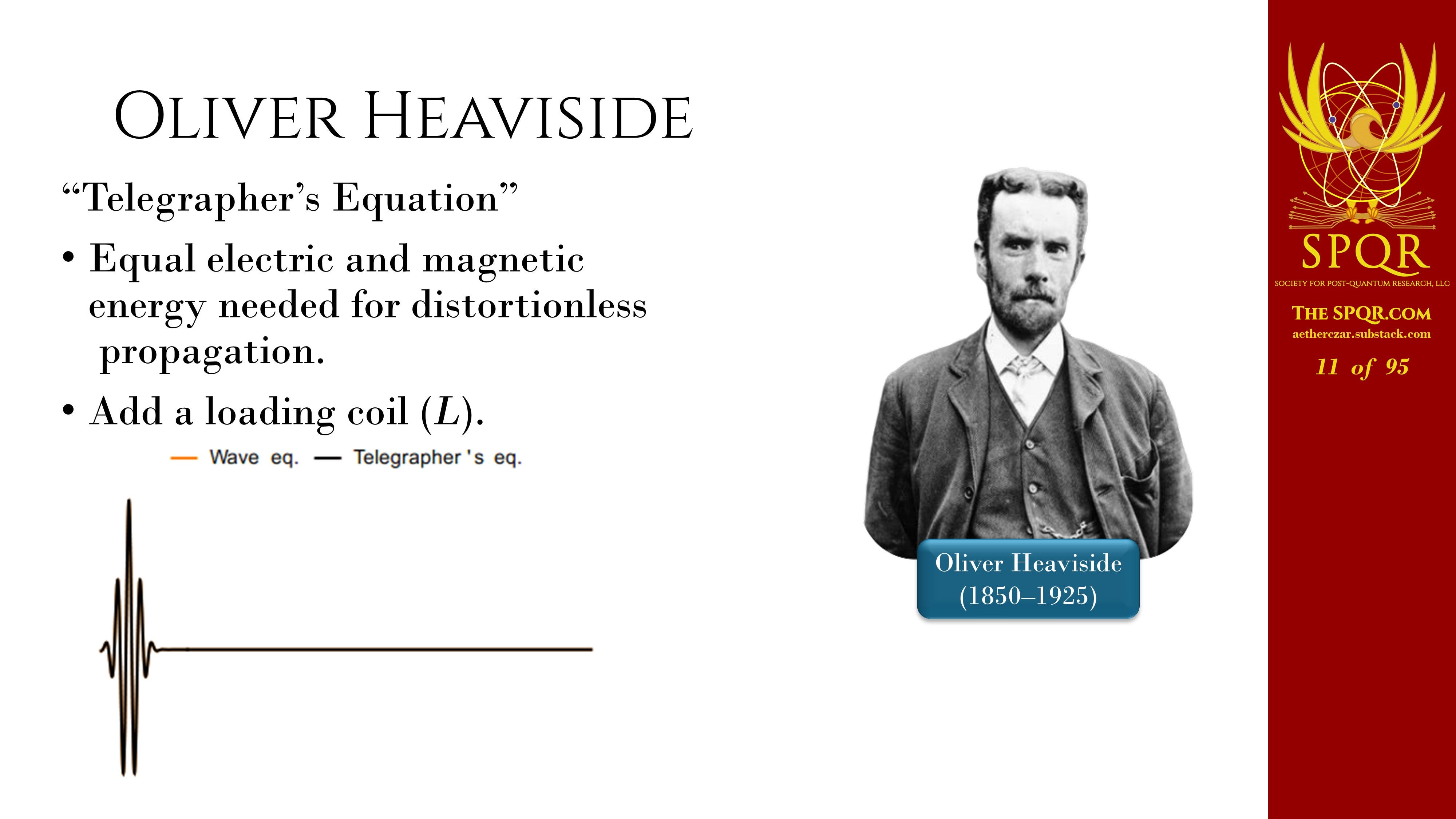
The key insight that Heaviside had is that an electromagnetic wave has a balance of electric and magnetic energy.

Heaviside’s “Telegraphers’ Equations” not only describe how dispersion distorts a signal, but also how to control cable parameters to achieve ideal wave propagation. Courtesy Jacopo Bertolotti.

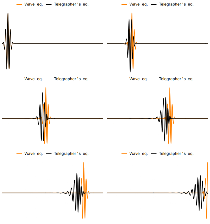
The transmission lines of the day tended to be capacitive. They were overly electric. So by putting a loading coil, adding some induction or some magnetic energy, he was able to eliminate the distortion and send signals through the lines without problems.

Electromagnetic Energy Flow

Well, about the same time in the 1880s, John Henry Pointing came up with his rule for how fields guide energy, the Poynting vector.

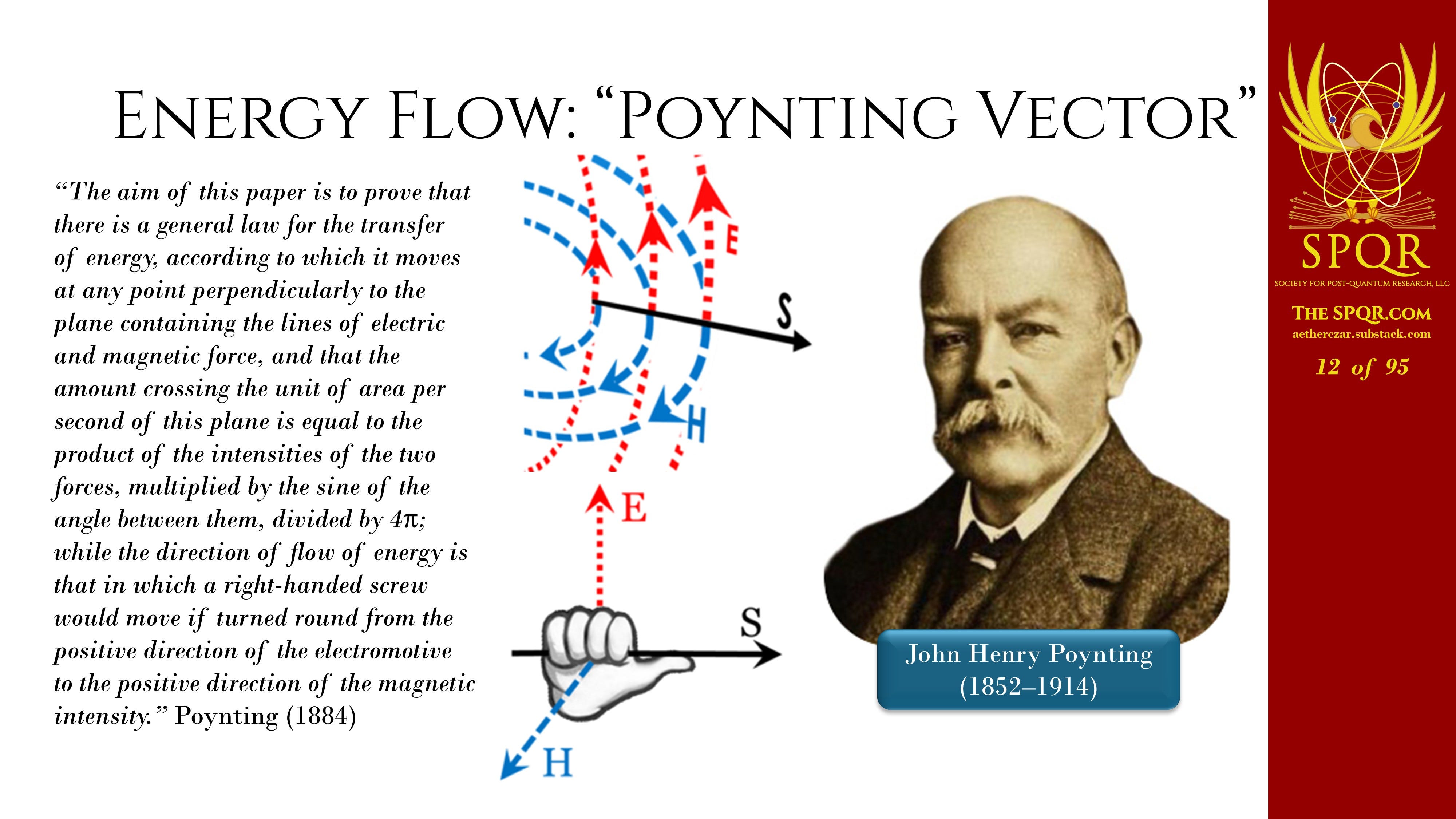
And I’ll spare you the wall of text about right-handed screws and which direction they’re turning, all of that was encapsulated in Heaviside’s much simpler vector format.

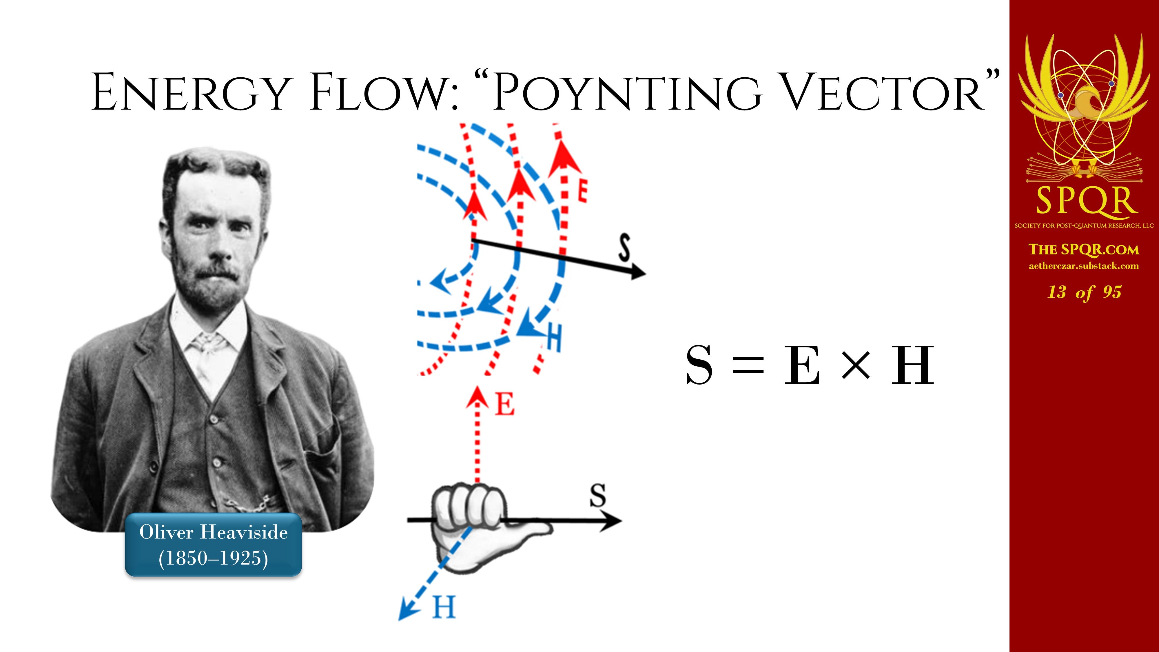
The Poynting vector equals the cross product of the electric field and the magnetic field — a relation that we still use today.

Heaviside commented that when energy goes from place to place, it has to traverse the intermediate space. He gave this physical interpretation of these laws of electromagnetic energy transfer.

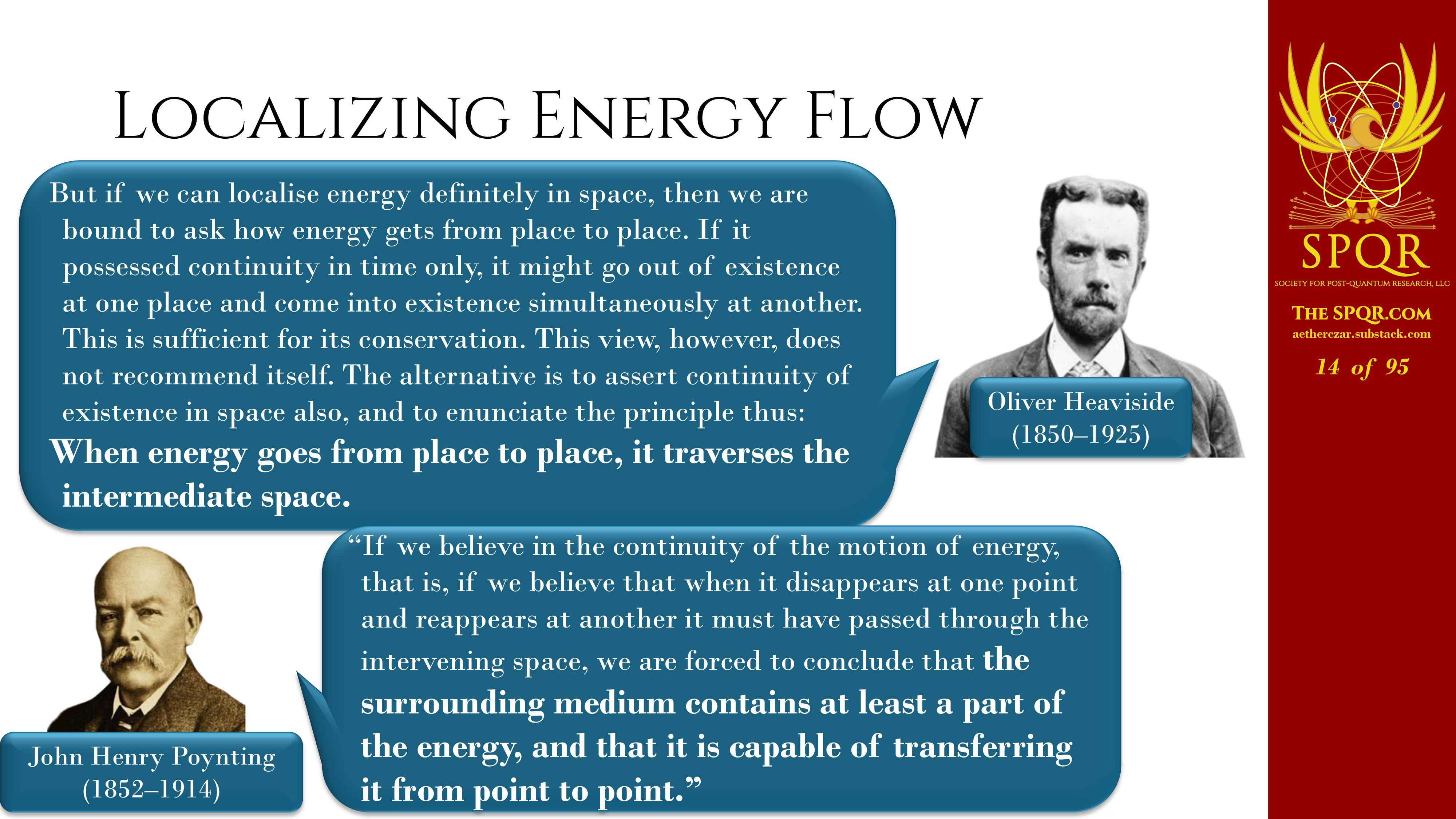
Similarly, Pointing commented that the surrounding medium has to contain part of the energy and it’s capable of transferring it from point to point. These weren’t just ad hoc additions that Heaviside and Poynting were making.

It goes back to Maxwell himself, who insisted there had to be a medium or substance in which the energy exists after it leaves one system and before it gets to another one.

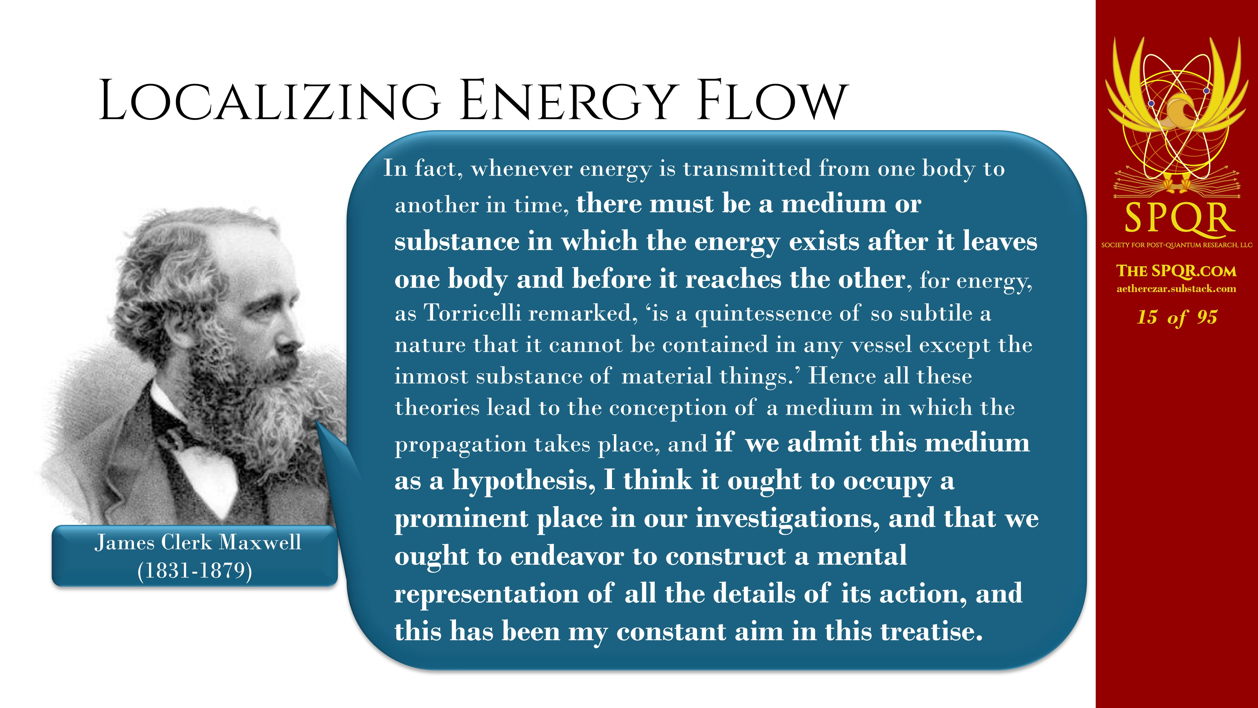
He added, I think this medium as a hypothesis ought to occupy a prominent space in our investigations, and we ought to endeavor to construct a mental representation of it, and that has been his constant aim in his treatise on electricity and magnetism.

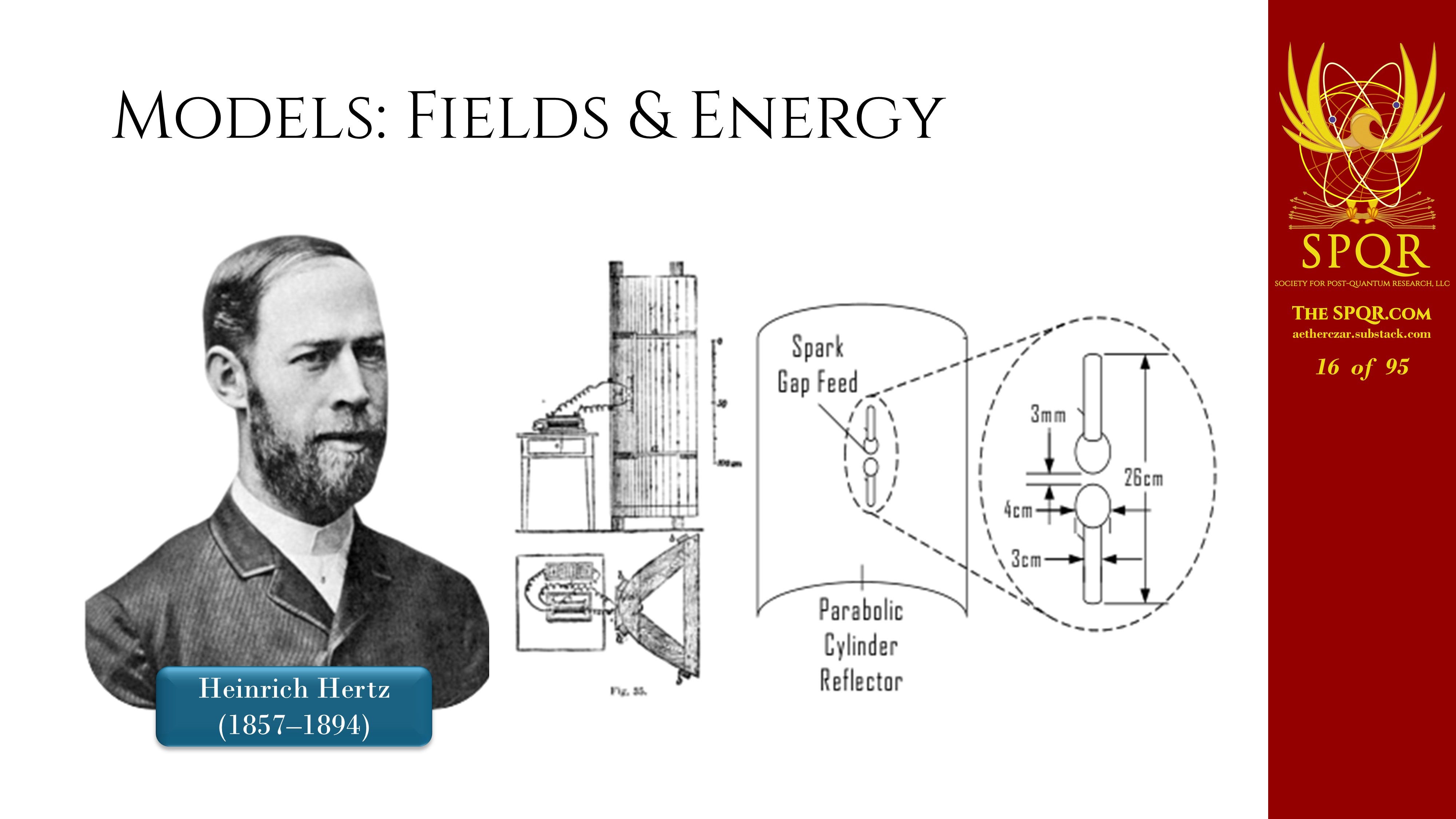
Well, along came Heinrich Hertz, who did experiments that caught electromagnetic waves in the act of moving from place to place. But Hertz was more than just a brilliant experimentalist. He was an excellent theoretician as well.

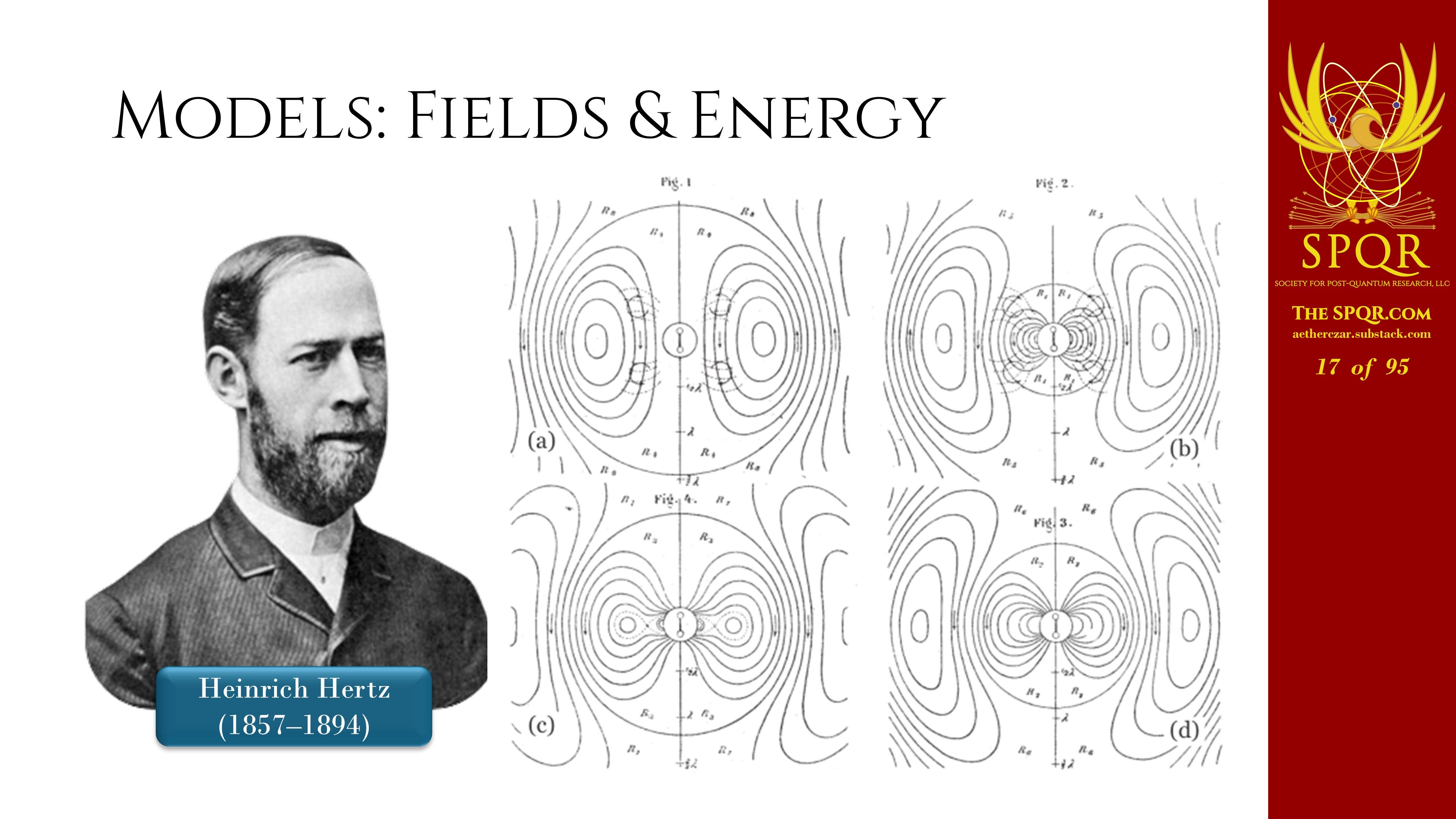
He created these diagrams of the dipole field and worked out the equations that describe how dipoles work.

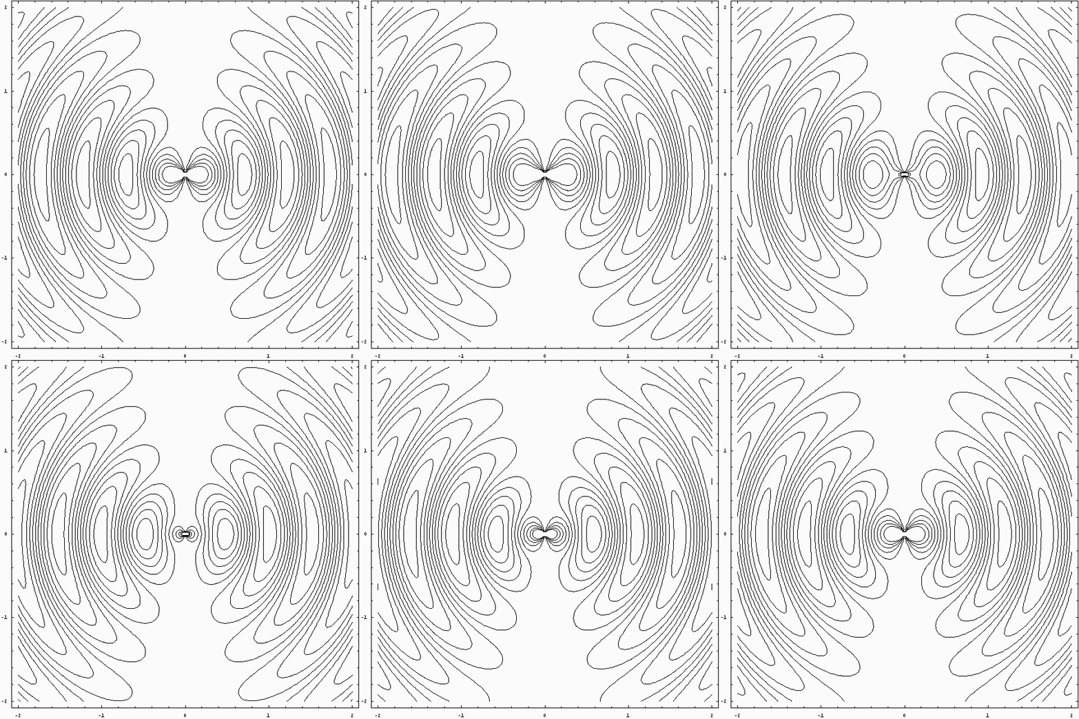
How an oscillating charge distribution or an oscillating current segment gives rise to the dipole fields. Schelkunoff and Friis some 70 or 80 years later would comment that the dipole equations that Hertz discovered are “the most fundamental and important equations in antenna science.”

What Went Wrong?

So what went wrong with this brilliant start to our understanding of electricity and magnetism?

Well, the first thing that happened is this guy, William Crooks, invented this marvelous thing called a Crooks tube, the first cathode ray tube. And J.J. Thompson used that cathode ray tube to discover the electron.

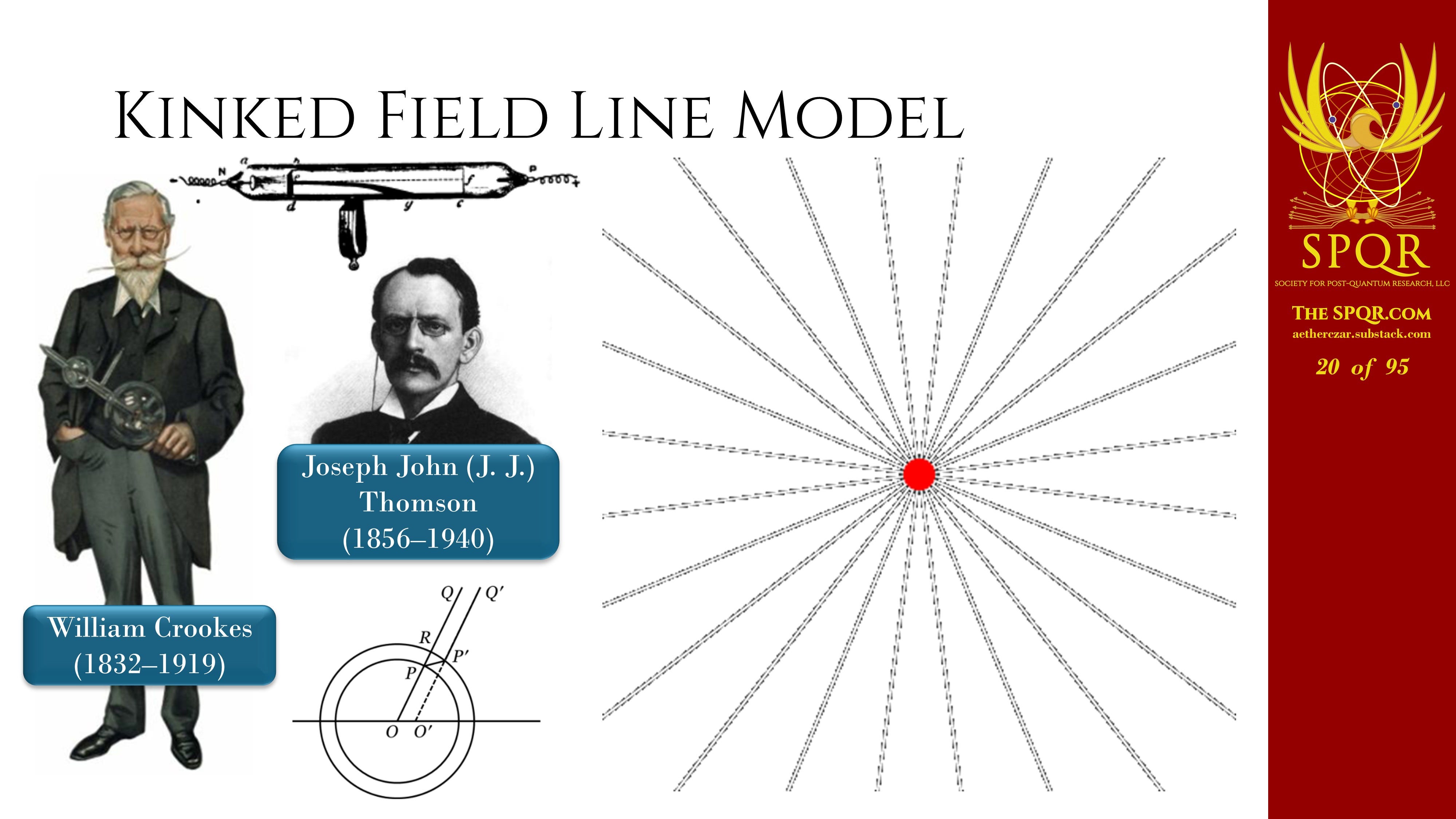
So, after the discovery of the electron, everyone was fascinated that we’d reduced electricity and magnetism to atoms of electricity.

People started thinking in terms of charges as being the fundamental entity that we’re dealing with in electricity and magnetism. If you have the radial field lines extending from your charge and you start to move it, the change in that radial field line propagates outward at the speed of light.

Radiation as a kinked field line from an accelerating charge, courtesy CalTech.

You get the transverse kinks that you see in the radial field pattern and that basically radiation is a kinked field line. Well, that model, the model of a single charge radiating, has really taken hold in a lot of thinking about how electricity and magnetism work.

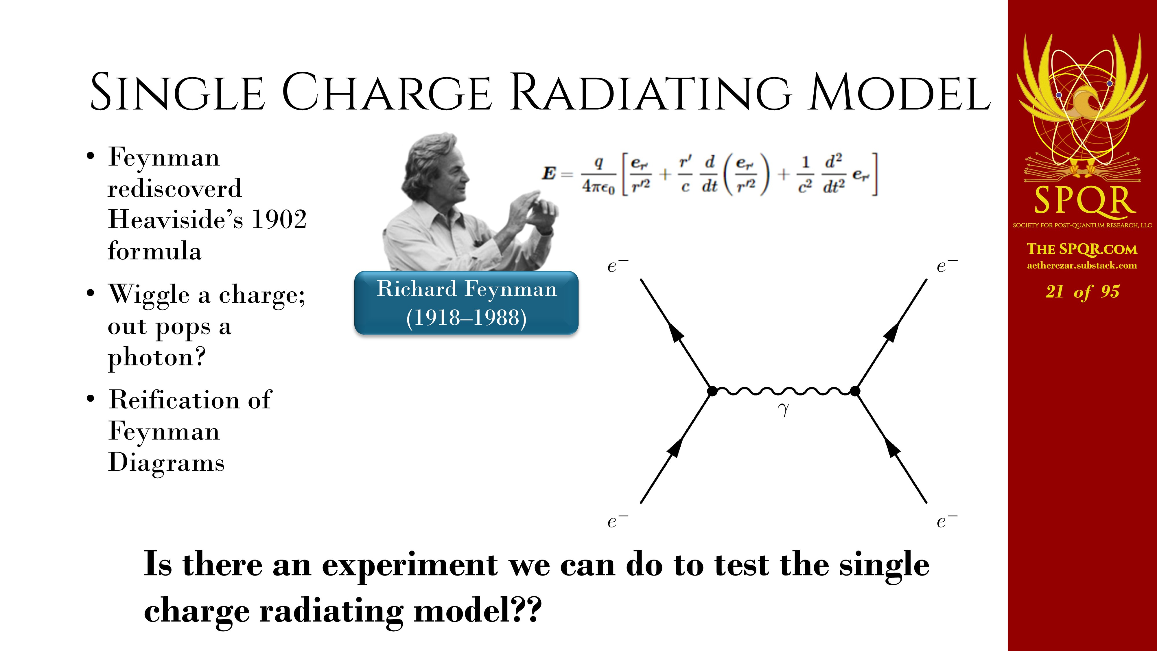
Feynman, for instance, rediscovered a formula that Heaviside had originally derived back in 1902 [Yes, I know Feynman says “1902,” and I said it too. It’s really “1904.” More about that some other time.] about the basic picture that you get when you take the Feynman diagrams that he came up with to keep track of terms in the power series involved in quantum electrodynamics, the basic picture you get is you wiggle this charge and out pops a photon from the charge.

Question is, is there an experiment that we can do to test or to validate this model of the single charge radiating? And it turns out there is a very simple experiment, and we can do this experiment right here in this ballroom.

If you hold your hand very steadily right out in front of you and slowly move it until you touch an object, your thigh, your chair, your neighbor, but only with your neighbor’s permission, what happens?

If the single charge radiating model is correct, there’s an issue called the issue of radiation reaction. The moment you started your hand in motion, what would happen is those accelerating charges would accelerate more and more and more and radiate more energy until they collided with the thigh and the result was the entire earth exploding. Well, clearly that didn’t work. There’s a problem with this model.

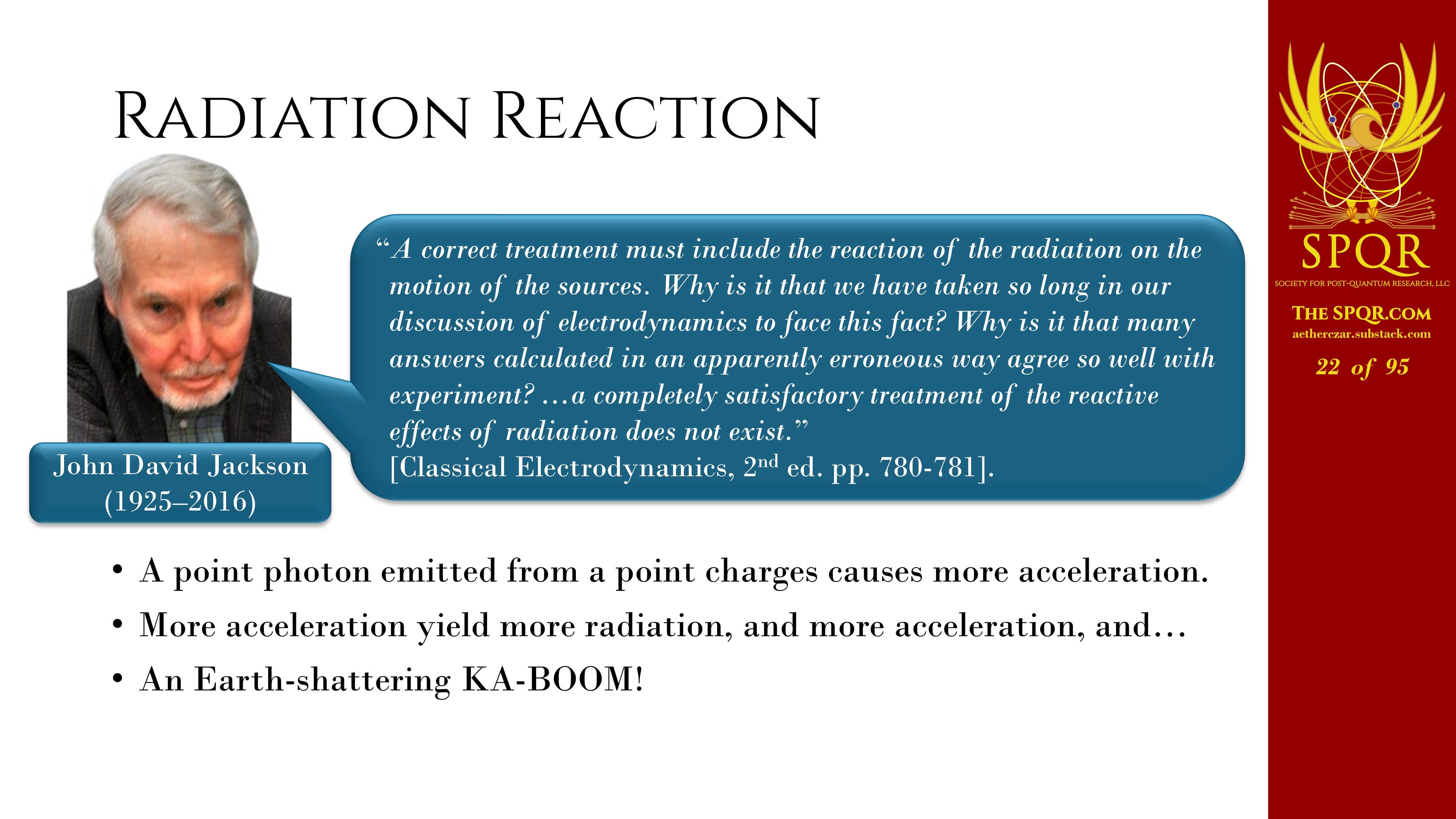
If you have a point photon emitted from a point charge, the fields act so as to cause more acceleration, which means more radiation, which means more acceleration. You get this exponential runaway. This is a problem that’s acknowledged, for instance, by J.D. Jackson, who wrote the book Classical Electrodynamics, the classic physics textbook on the subject.

So we should have seen an earth-shattering kaboom.

And the question is, where’s the kaboom? Why didn’t we see a kaboom? And the answer is, the single charge radiating model is fundamentally wrong. And you can understand that by reference to Zen Buddhism.

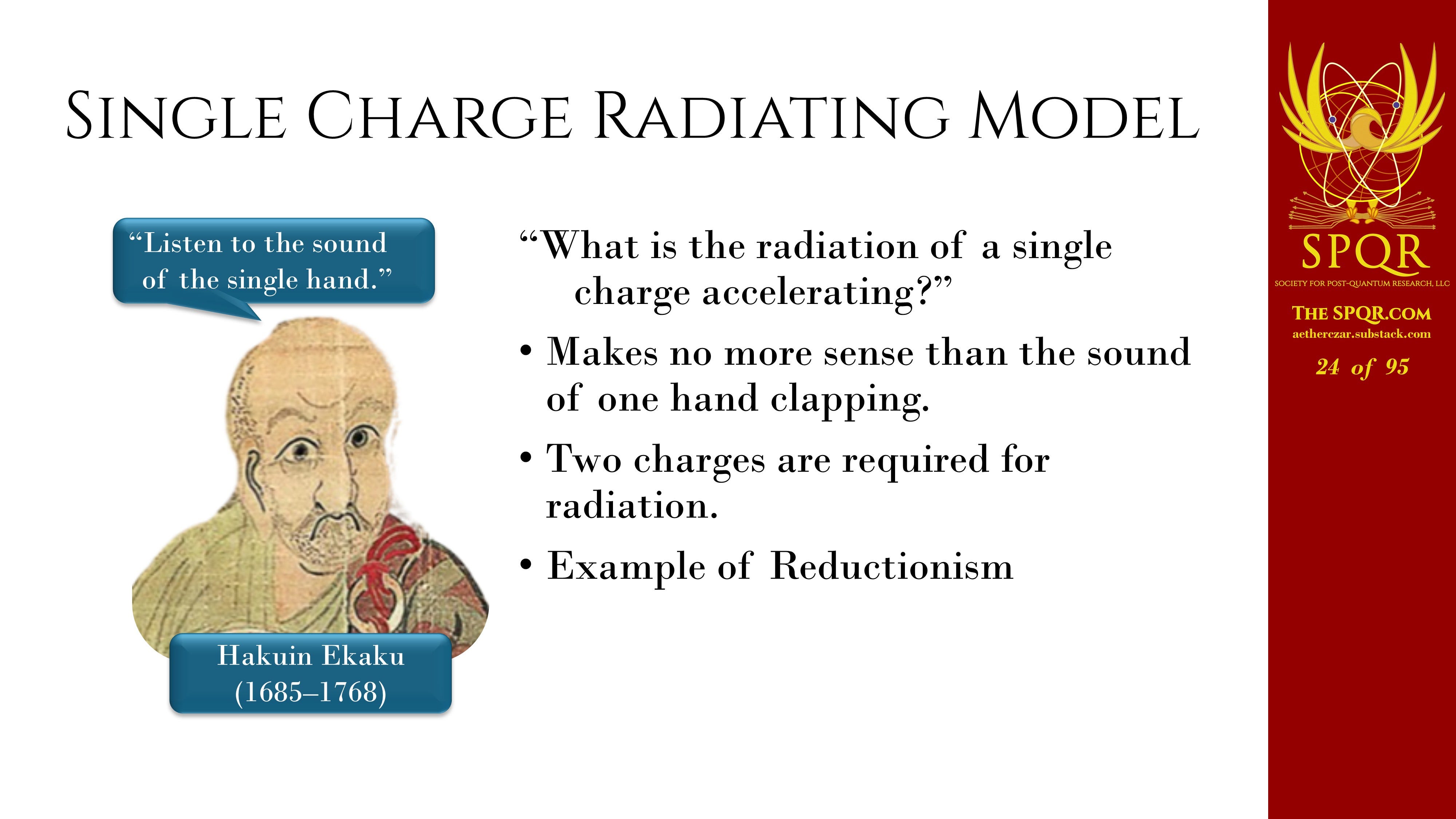
The Zen master Hakuin Ekaku advised his young acolytes to try to listen to the sound of a single hand clapping. Well, we know that’s a nonsense concept. A single hand can’t clap. You have to have two hands in order to clap. And that’s the fundamental problem that’s wrong with the single charge radiating model. It takes two charges to radiate, at least like an equal and opposite charge and a dipole, or you have to have a charge distribution setting up a field to make your single charge radiating. And if you try to consider that system in isolation, you get results every bit as nonsensical as the sound of a single hand clapping.

If you look at the acceleration of a single charge, what you find is if the charge is accelerating, its kinetic energy is increasing. It’s absorbing energy. Or equivalently, it’s a tiny little current segment, and the current’s getting bigger and bigger. It’s got more and more It’s absorbing that magnetic energy. An accelerating charge absorbs energy. It does not emit energy.

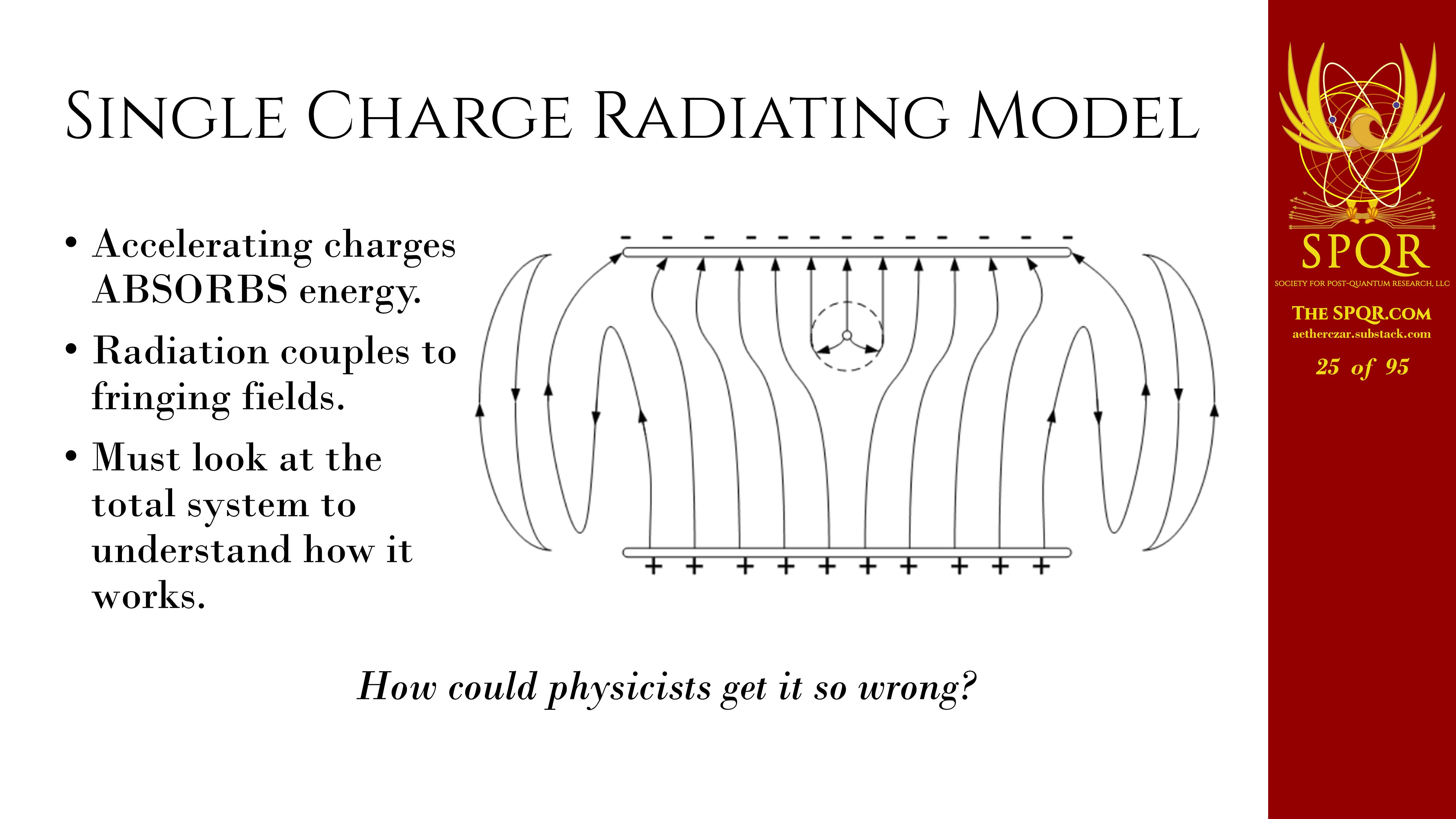
The energy that is radiated comes from the fringing fields of the capacitor giving rise to the charge distribution. The radiation fields propagate out through the inward flux of energy. And then only couple to the energy stored in the fringing fields to radiate away. You have to look at the totality of the system to understand what’s going on and not just focus on that single charge and try to model it.

And that’s why we don’t get the earth shattering kaboom… fortunately.

So how could physicists get it so wrong?

Part of the reason is a disdain for philosophical considerations. In fact, Neil deGrasse Tyson a few years ago was interviewed on a podcast, and he said, “the scientist knows when the question, what is the sound of one hand clapping, is a pointless delay.”

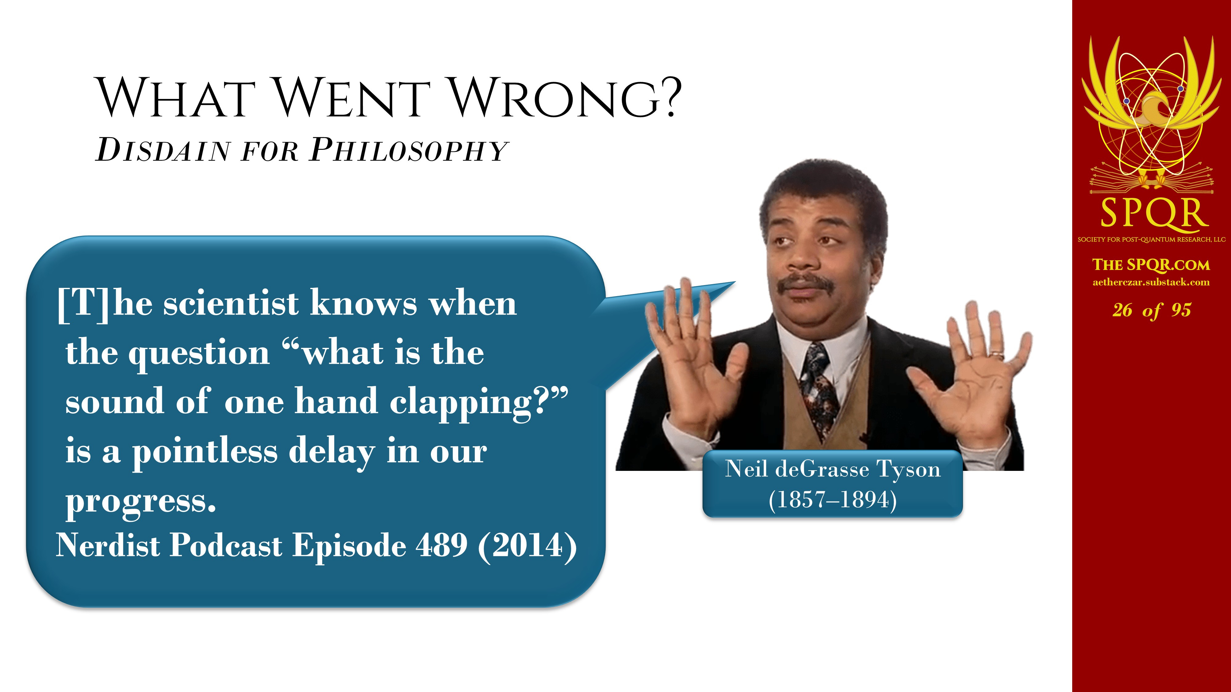
Well, it turns out that’s the exact philosophical premise you’ve got to understand to appreciate what’s wrong with a single charge radiating model. But we can go back more fundamentally and take a look at the conventional wisdom.

Correction: I listed Neil deGrasse Tyson (1857–1894). This appears to have been a serious error in my choice of reference frame. I am reliably informed that Tyson was born in 1958 and remains very much among the living. I regret having prematurely consigned him to the history of science.

The Conventional Wisdom

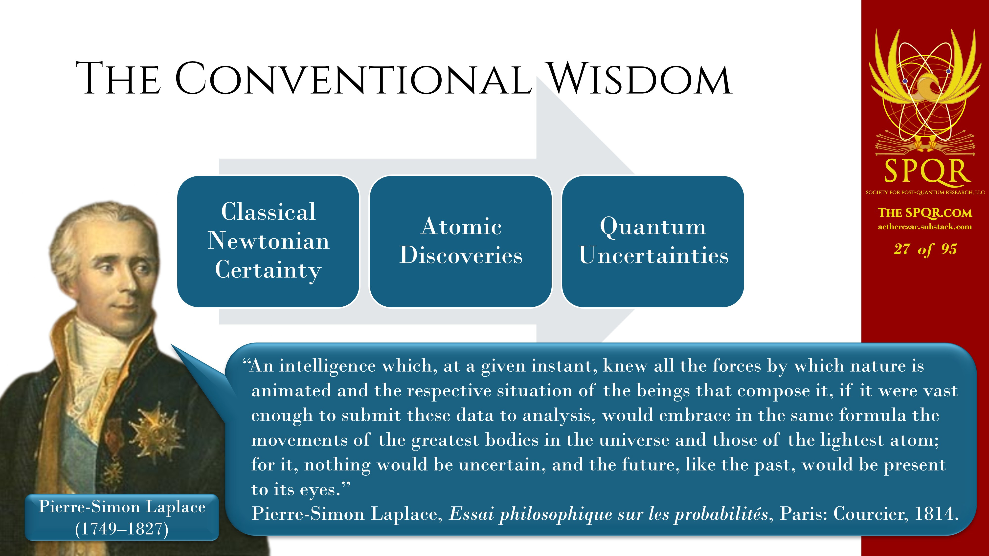
We started with what has been called classical Newtonian certainty as encapsulated in by Pierre Simon Laplace who commented that if only we knew the location of every particle in the universe and all of its velocities and all the forces and accelerations on it, in principle we would be able to know the, have absolute certainty on the unfolding course of events. Well, the discoveries of quantum mechanics and atomic physics in the 1920s suggested that perhaps reality was not causal, that it could not be predicted.

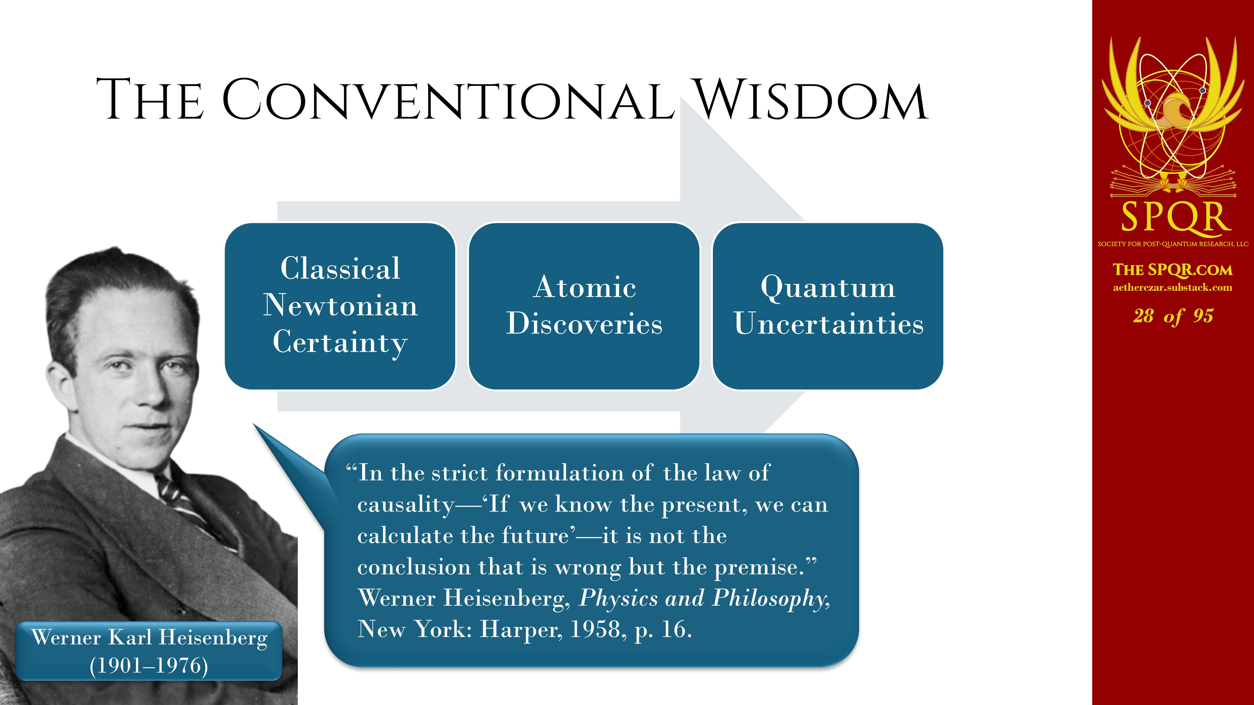
That’s encapsulated here by Heisenberg’s comment that the strict formulation of the law of causality is fundamentally wrong.

What Really Happened?

Well, that happened because the key experiment that was involved there was Michelson and Morley and their work on an interferometer to try to detect the motion of the earth through the ether. They came up with a result.

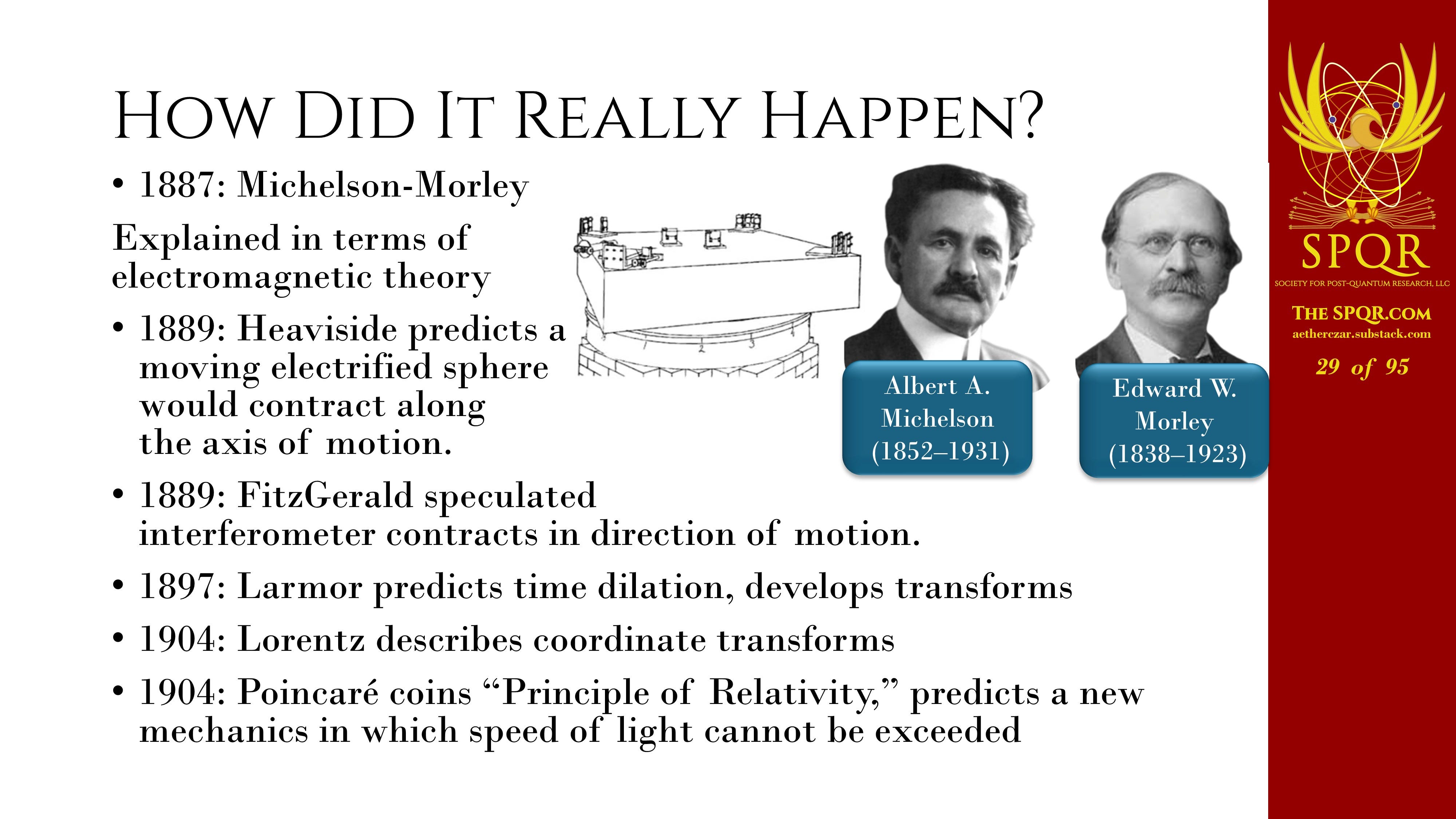
That was a result that was far less than they would have expected if they were looking at the Earth’s motion. That was explained in terms of electromagnetic theory by a variety of people who followed in his footsteps, culminating in Poincaré, who in 1904 coined the term “principle of relativity,” and he predicted a new mechanics where the speed of light could not be exceeded.

That bottom-up approach to understanding the electrodynamics of moving charges got called into question by a young Swiss patent clerk named Albert Einstein.

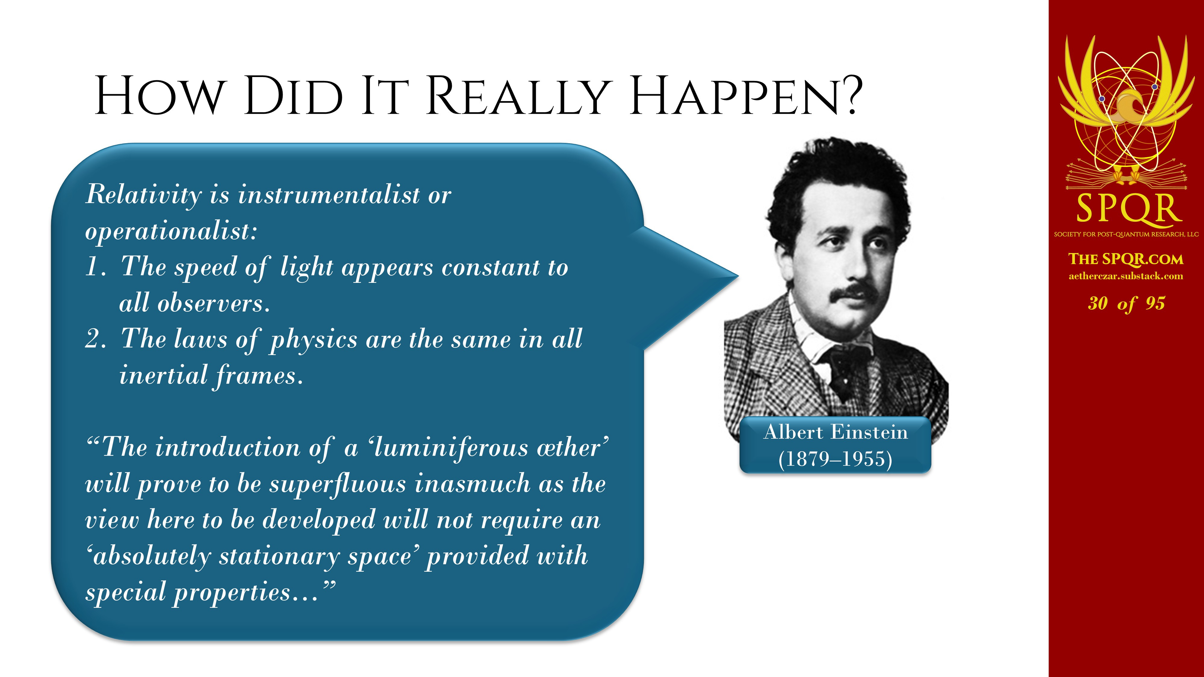
He took what’s called an instrumentalist or an operationalist approach influenced by Ernst Mach where he focused on, well, what are the observations and what does the observer see? And he pointed out the observer sees the speed of light being constant and the laws of physics the same in all inertial frames. And he argued that that gave all of the Lorentz transforms and the laws of the motion of a classical charge and that therefore any concept like an aether was completely superfluous and unneeded.

Fast forward 10 years and Einstein is developing the general theory of relativity. John Wheeler commented that you can think of that theory as space-time telling matter how to move and matter telling space-time how to curve.

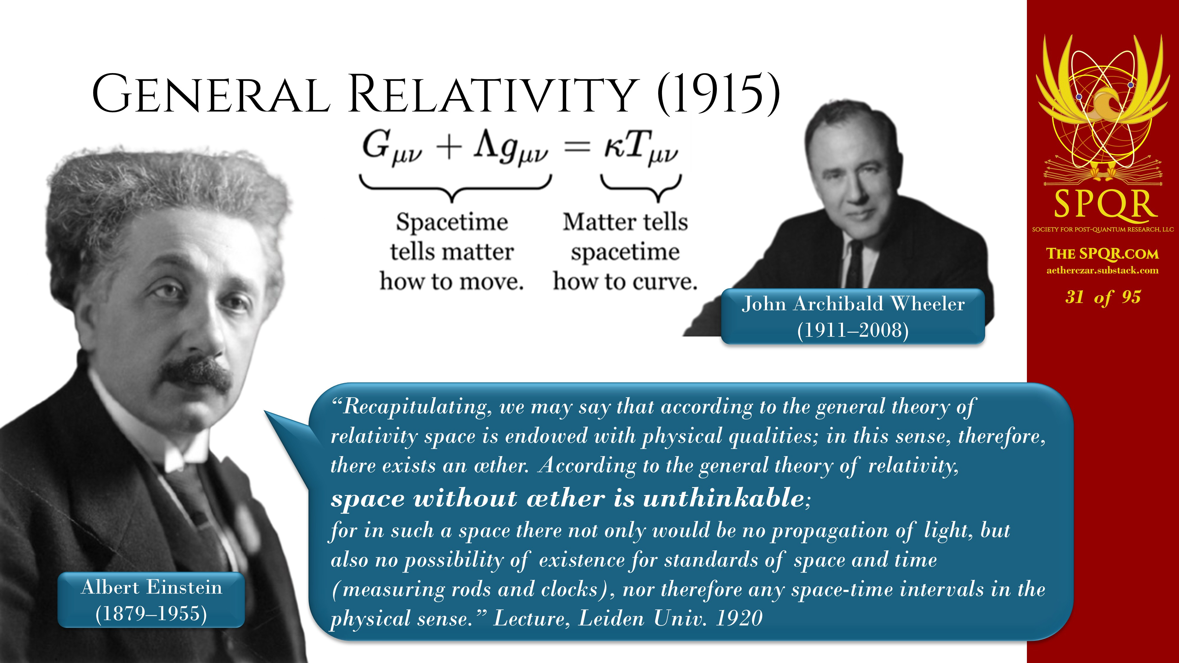
Curvature of space-time got Einstein thinking and backing away from his purely observation-based approach to physics. He argued in a speech five years later in 1920, space without aether is unthinkable. Somehow space possesses this property of curvature that’s necessary for general relativity to work.

Well, fast forward another five years, and Heisenberg is giving his first lectures on quantum mechanics in Berlin. According to Heisenberg, writing in his memoirs in 1970 or so, 15 years after Einstein’s death, Einstein invited Heisenberg back to his apartment.

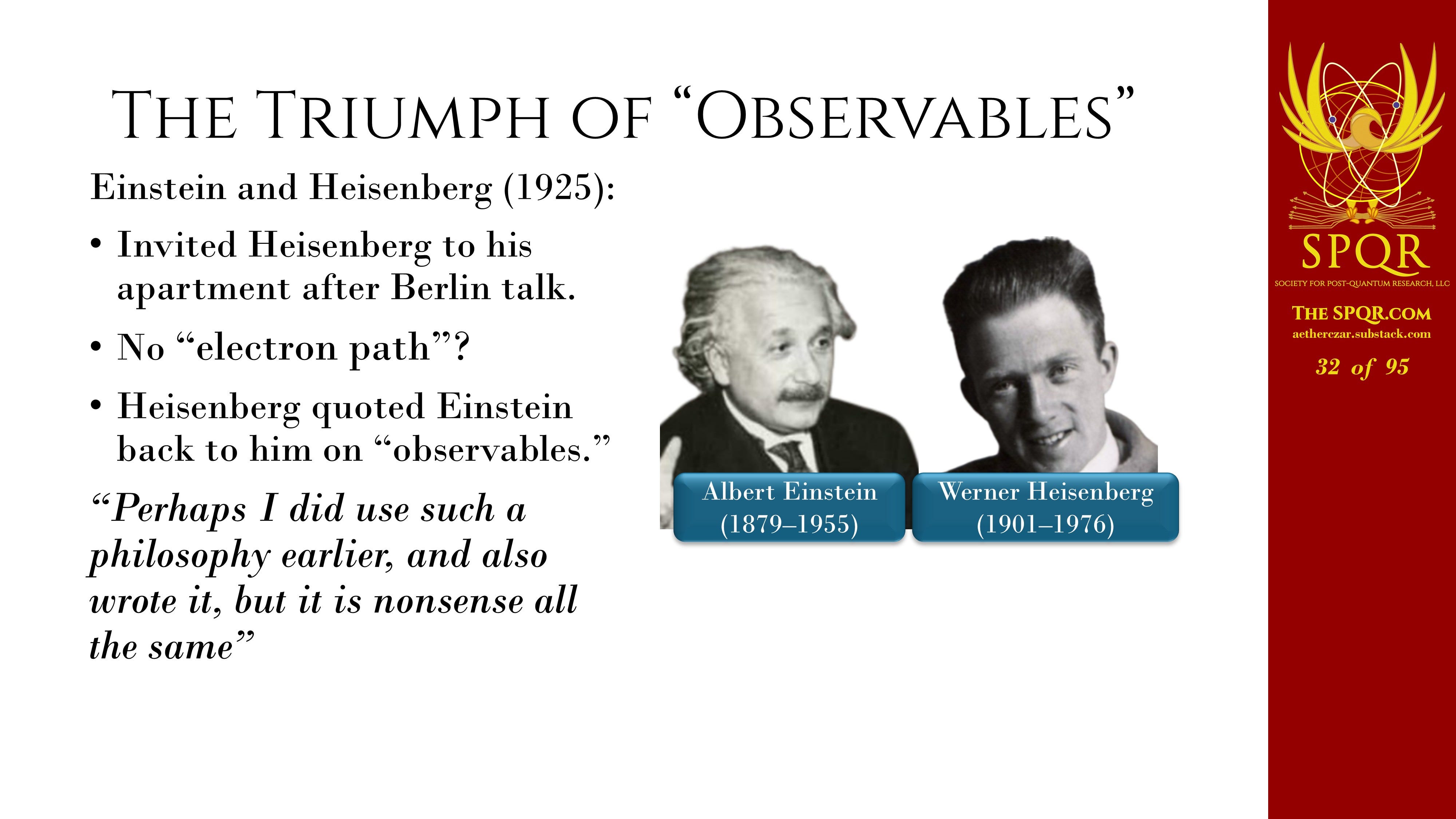
And Einstein said, “Well, wait a moment, the electrons have got to be in there somewhere. How do you deal with this?”

And Heisenberg proceeded to quote Einstein back at Einstein on the importance of focusing on observations and how theories should only deal with what the experimental measurements are observing. And according to Heisenberg, Einstein finally conceded and said, “well, perhaps I did use such a philosophy earlier and even wrote it, but it’s all nonsense just the same.”

And that was really Einstein’s break with a conventional Copenhagen interpretation. Of quantum mechanics. But this idea was pretty common. It wasn’t just Einstein who brought the idea into physics. A whole host of his contemporaries all were arguing that causality has nothing to do with the business.

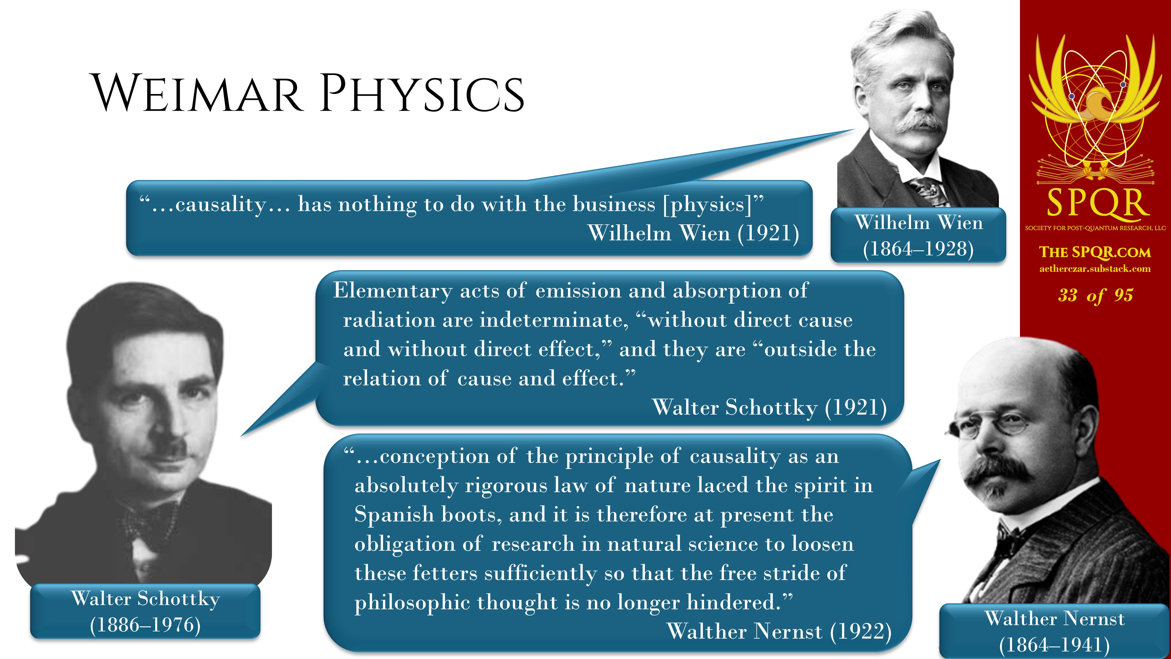
Or that acts of emission absorption of radiation are without direct cause and without direct effect. Or that the causality needs to be abandoned so we don’t fetter the spirit in Spanish boots.

In 1927, the Fifth Solvay Conference, there was a very famous exchange between Einstein and Bohr where Einstein argued that God does not play dice with the universe. And according to legend, Bohr’s response was to tell Einstein to stop telling God what to do. That conflict overshadowed something else that was going on at the time.

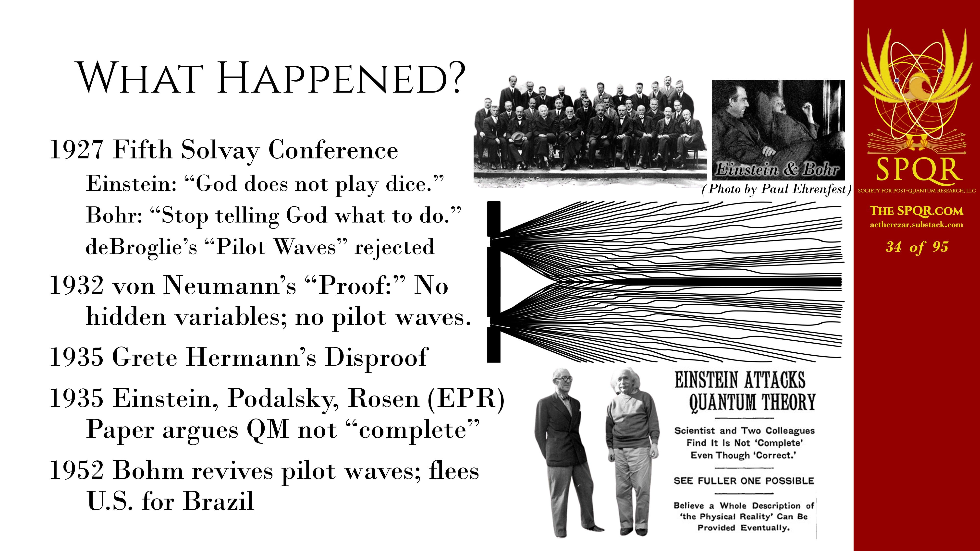
A Frenchman named Louis de Broglie had introduced the concept of pilot waves.

His argument was, if you had, say, a two-slit experiment, you had the wave propagated. Propagating through, going through the two slits, setting up an interference pattern, guiding the motion of a particle through one slit or the other slit. It was a deterministic theory of quantum mechanics. Well, that flew in the face of Bohr and the Copenhagen interpretation.

And it was largely rejected, and de Broglie was convinced to abandon that. In 1932, the famous mathematician John von Neumann came up with a mathematical proof that there could be no hidden variables, that a de Broglie-like theory could not possibly be valid. Just a few years later, a mathematician and philosopher named Greta Hermann disproved that, but no one paid any attention to her.

In 1935, Einstein and his colleagues Podolsky and Rosen wrote what came to be known as the EPR paper arguing quantum mechanics is not complete and there had to be hidden variables.

Bohm Revives Pilot Waves

But it wasn’t until the 1950s that another physicist named David Bohm rediscovered and revived the de Broglie pilot wave theory. But unfortunately, he ended up suspected of communist sympathies and fled the country to Brazil to avoid any difficulties involved in that.

So he was at Princeton University at the time, and the head of the Institute for Advanced Studies was this guy, J. Robert Oppenheimer, more famously known as the director of the Manhattan Project. Oppenheimer was a big He did not like this pilot wave stuff that Bohm and de Broglie were advocating. So according to the story, he handed a graduate student Bohm’s paper and said, “Don’t come back until you’ve found something wrong with this.”

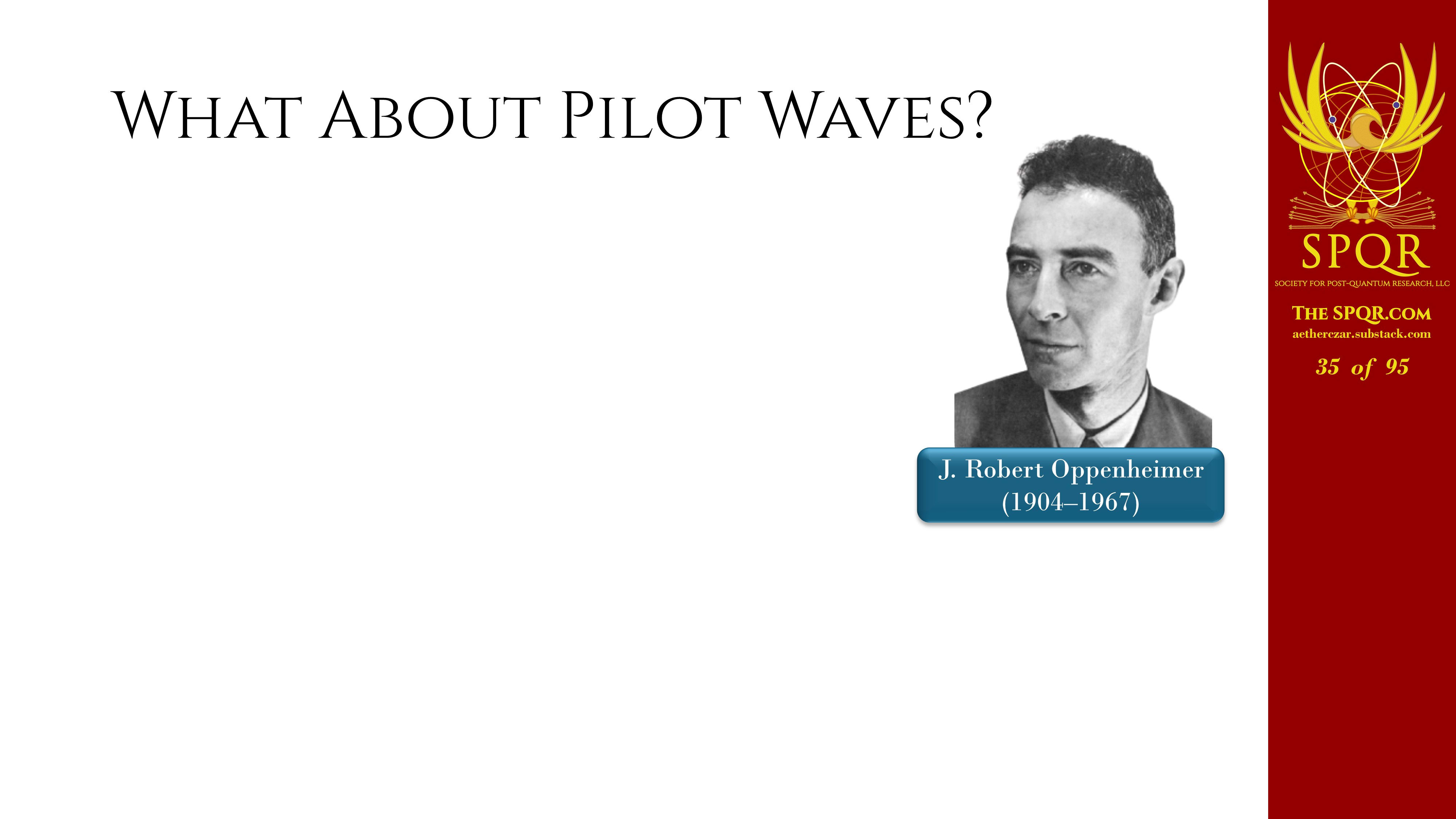
The graduate student sheepishly came back to Dr. Oppenheimer saying, “I’m sorry, sir, I can’t find anything wrong with this.” So with a sigh, Oppenheimer took it back and decided he’d have to just do it himself.

And he couldn’t find anything wrong with it, either.

So he convened a seminar at the Institute for Advanced Studies to assemble all the best and brightest minds at Princeton to finally put a stake through the heart of this heretical pilot wave causal theory of quantum mechanics. And at the end of the day, no one could find a technical flaw or reason to disprove the theory.

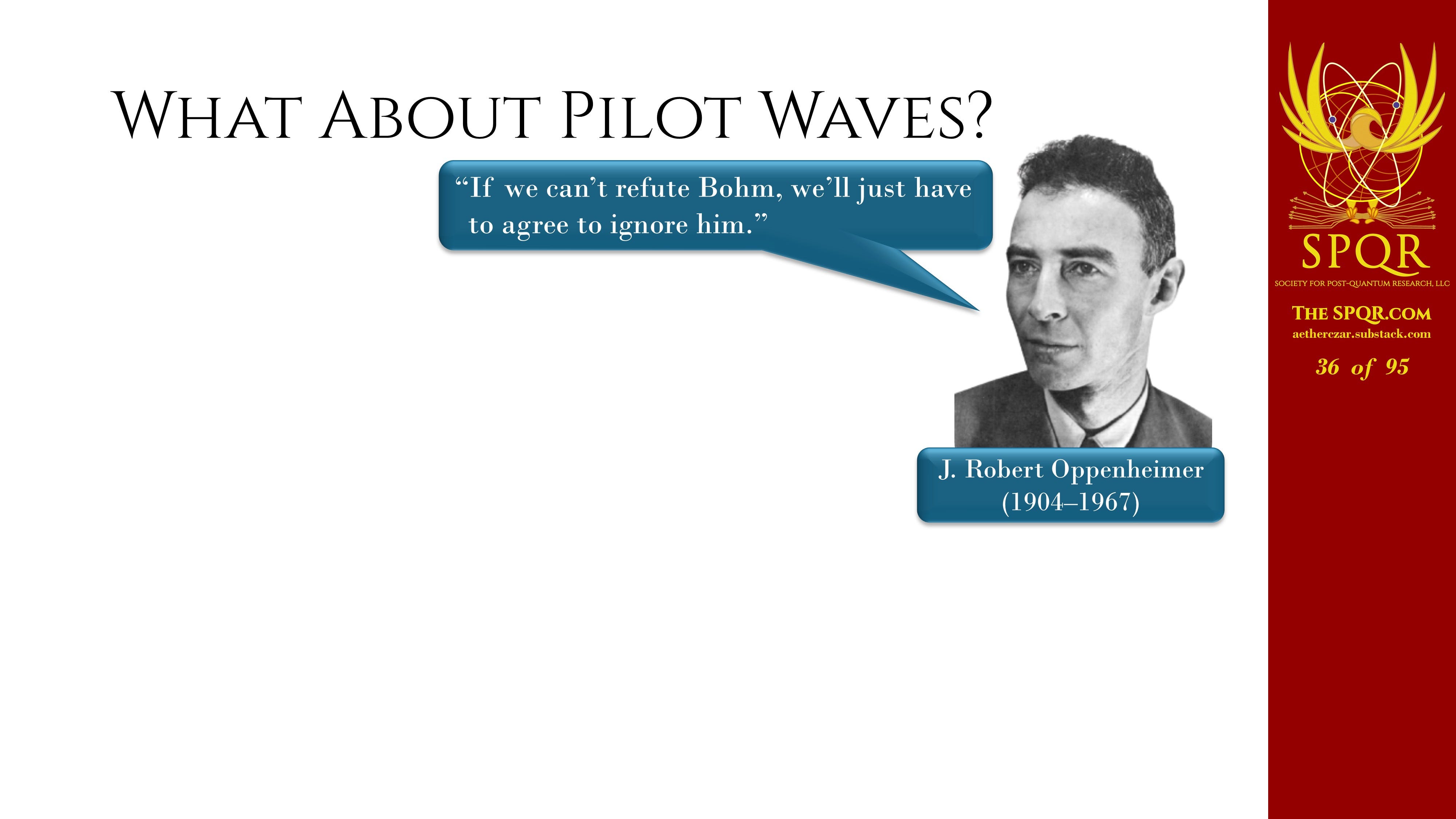
So according to one of the participants, Oppenheimer said, “Well, if we can’t refute Bohm, we’re just going to have to agree to ignore him.”

And you hear a story like that and that doesn’t sound like the way you’d expect scientists to be behaving.

And I’d have been kind of skeptical of that story too, if I hadn’t had a front row eyewitness opportunity to see something similar. When I studied physics down the road here at the University of Texas at Austin, I had the good fortune to have John Wheeler on my doctoral committee.

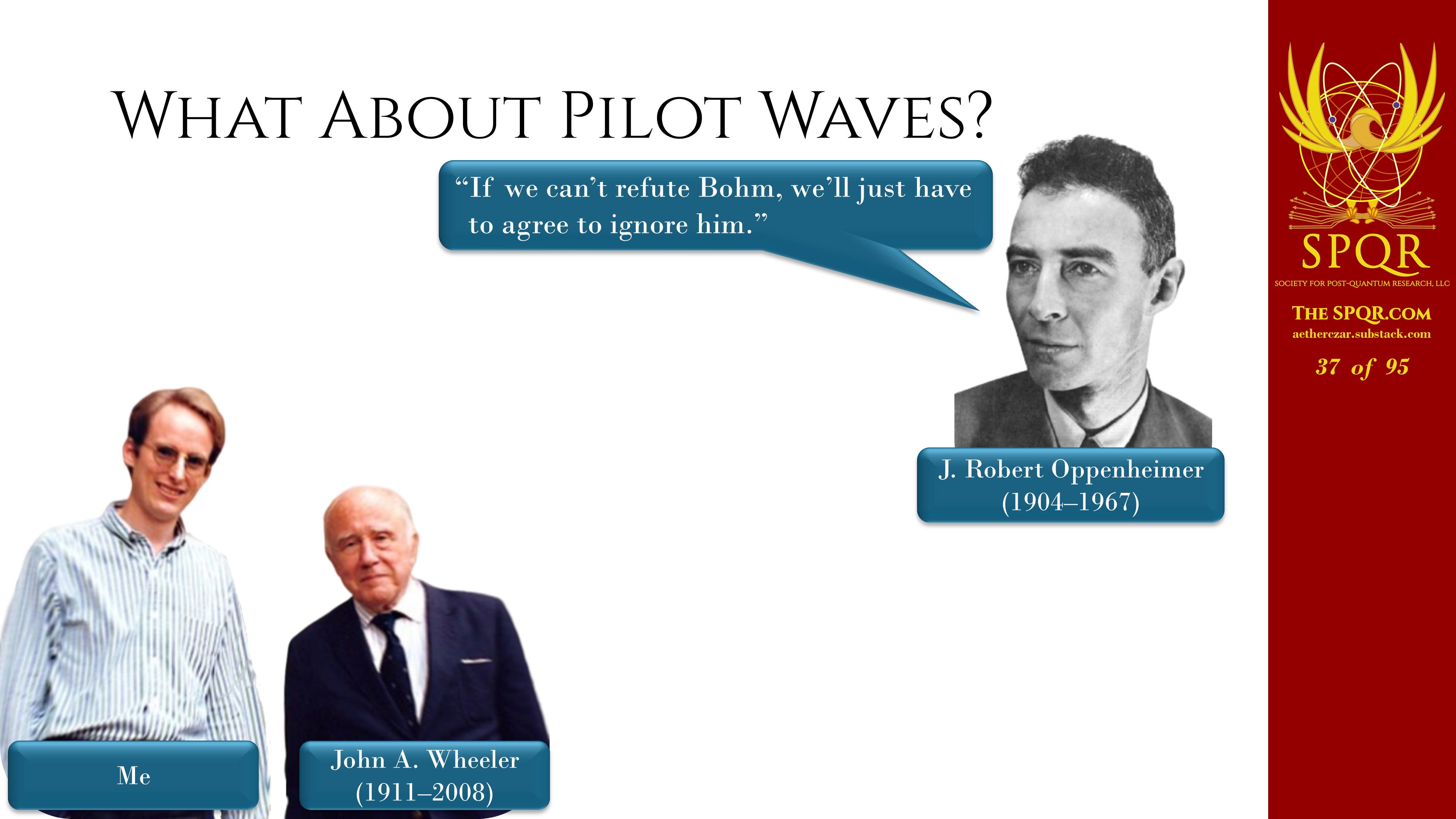
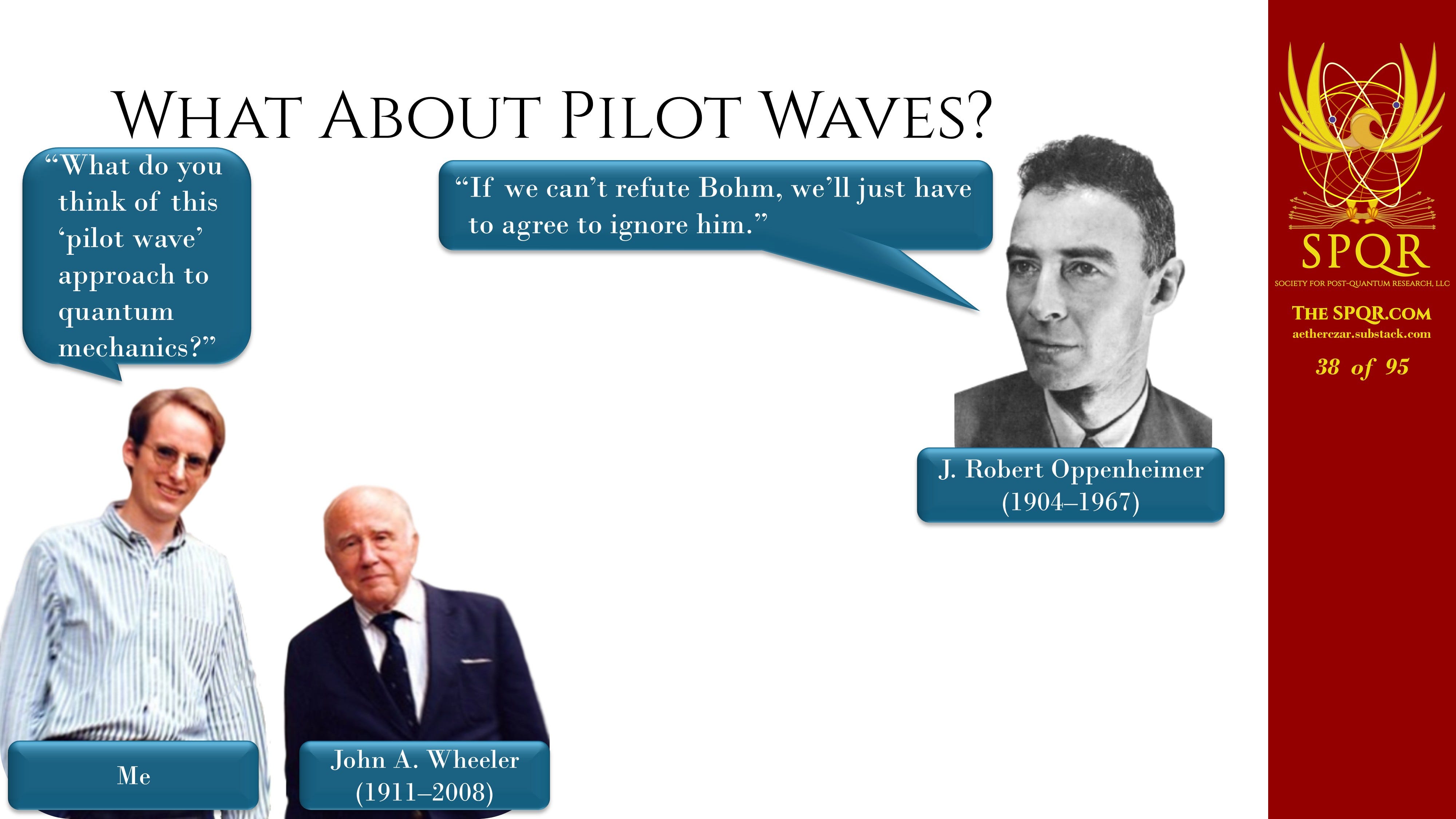
He had studied with Bohr. In addition to coining the term “black hole,” he did pioneering work in quantum measurement theory. So when I was befuddled by the whole Copenhagen approach to quantum mechanics that I learned in graduate school, and I finally discovered the pilot wave approach that made so much more intuitive sense, I took the opportunity to talk with Professor Wheeler about it. And I asked Professor Wheeler, “What do you think of this pilot wave approach to quantum mechanics?”

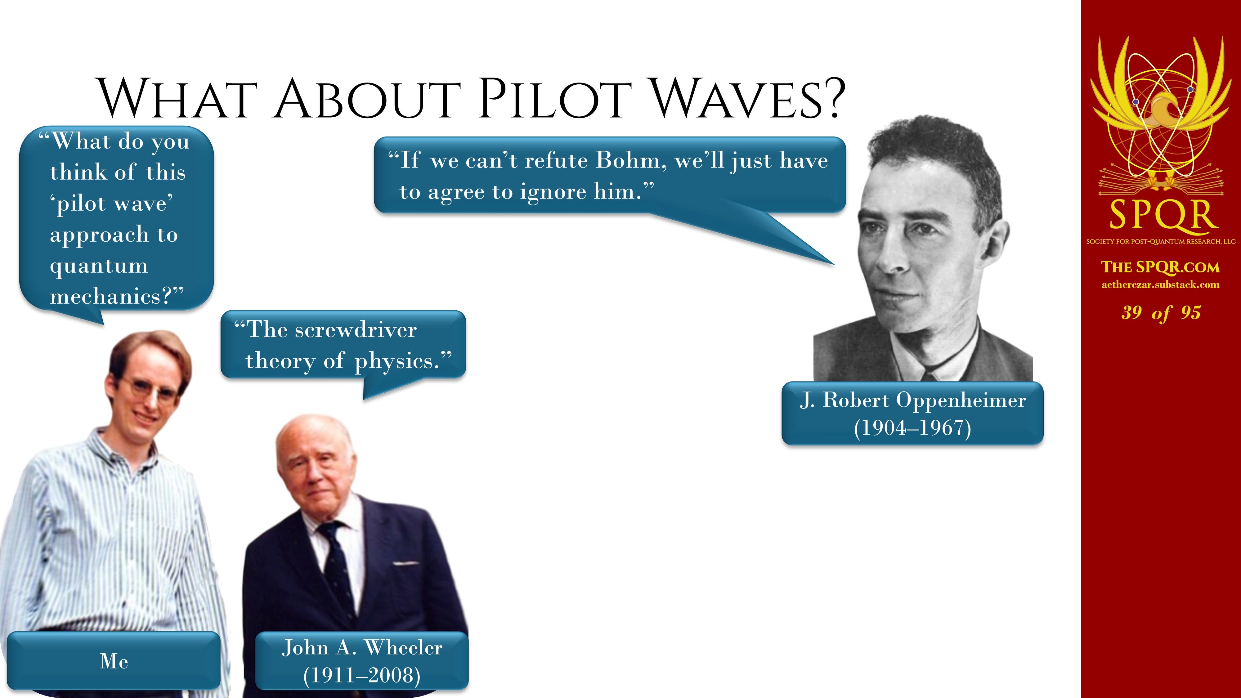
And he said, “AH! The screwdriver theory of physics.”

And I wasn’t quite sure what he meant by that, although it was obviously pretty derogatory. And so I asked him, well, have you written a paper or analysis? Is there someplace I can go to understand what your criticisms are and why you don’t like this approach to quantum mechanics?

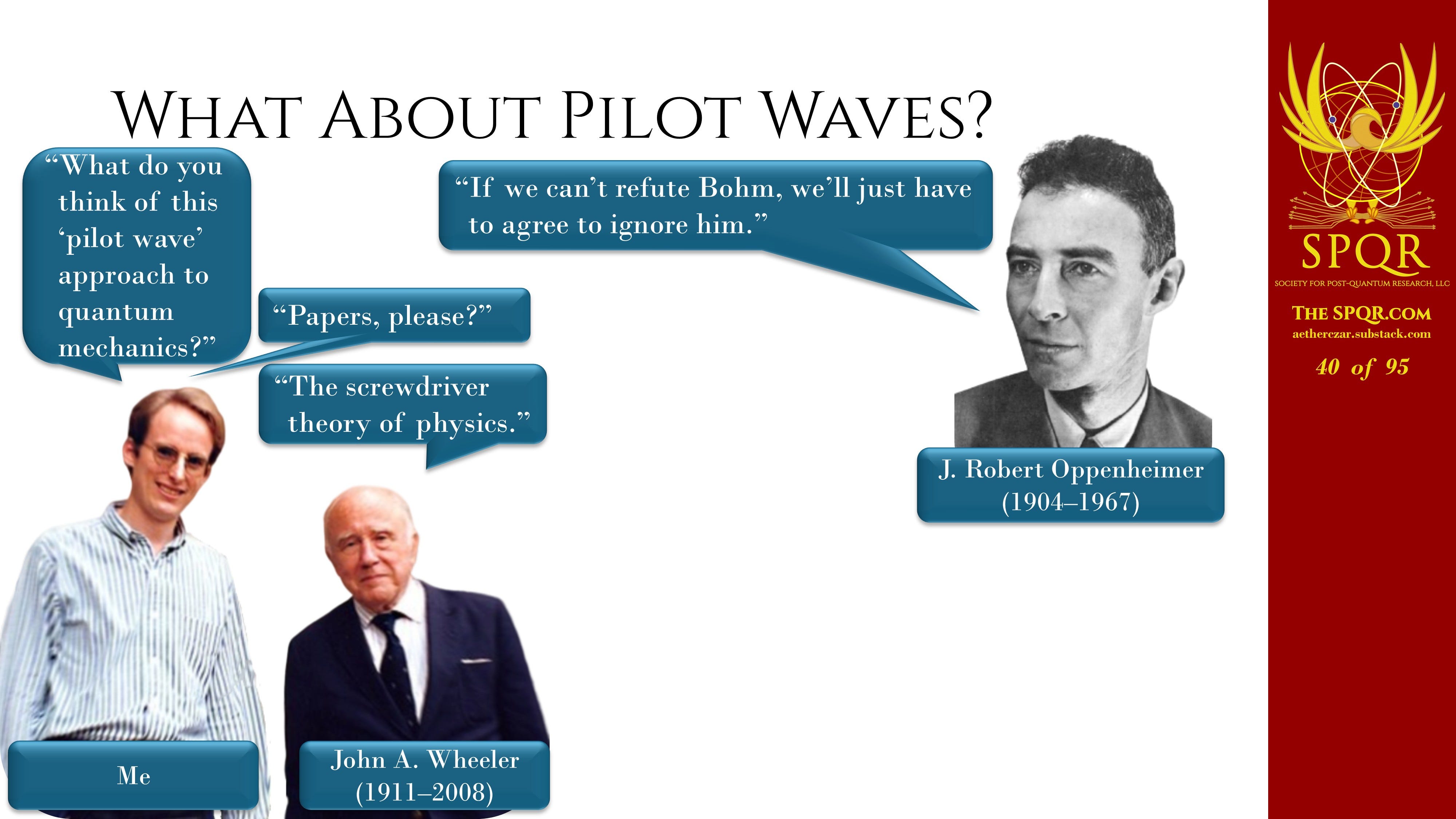
And he looked at me and he said, “You know, I never really studied into that business and I really should so I can see what’s wrong with it.”

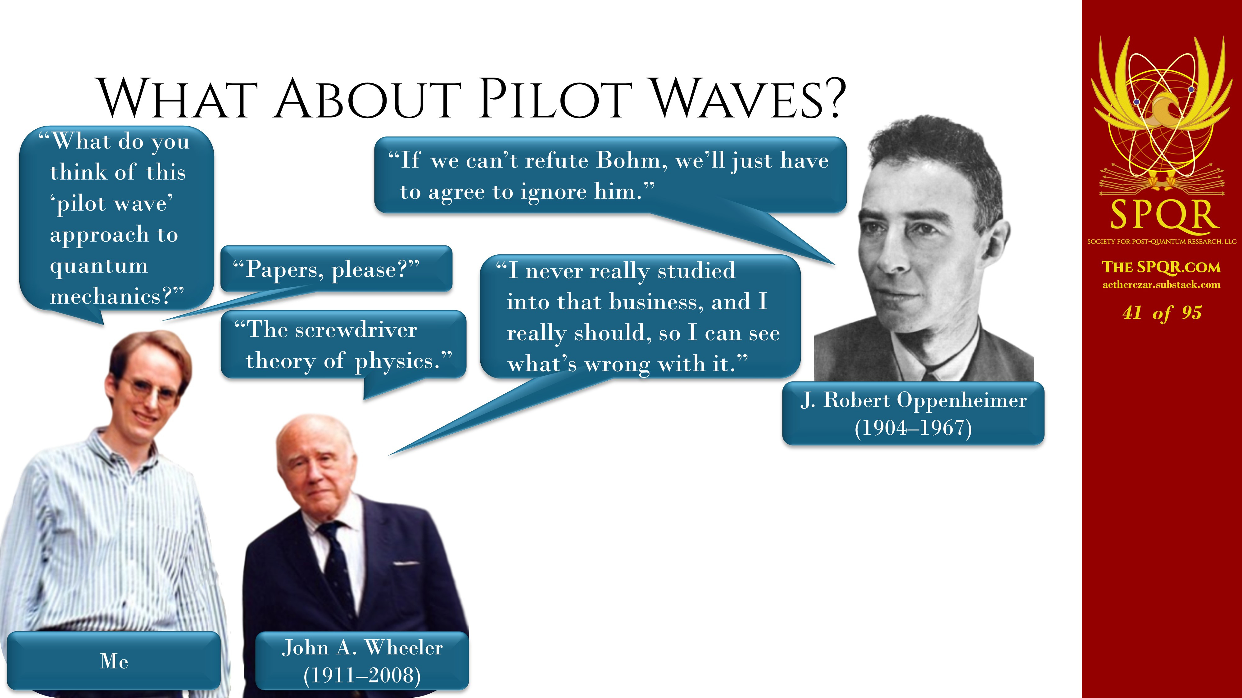
It was amazing to me that Wheeler would have that kind of an attitude, the blinders… he never seriously engaged with or tried to understand this fundamental alternative to quantum mechanics.

I discussed my experiences with John Wheeler, in this post.

And it really wasn’t until decades later that I realized the significance of this.

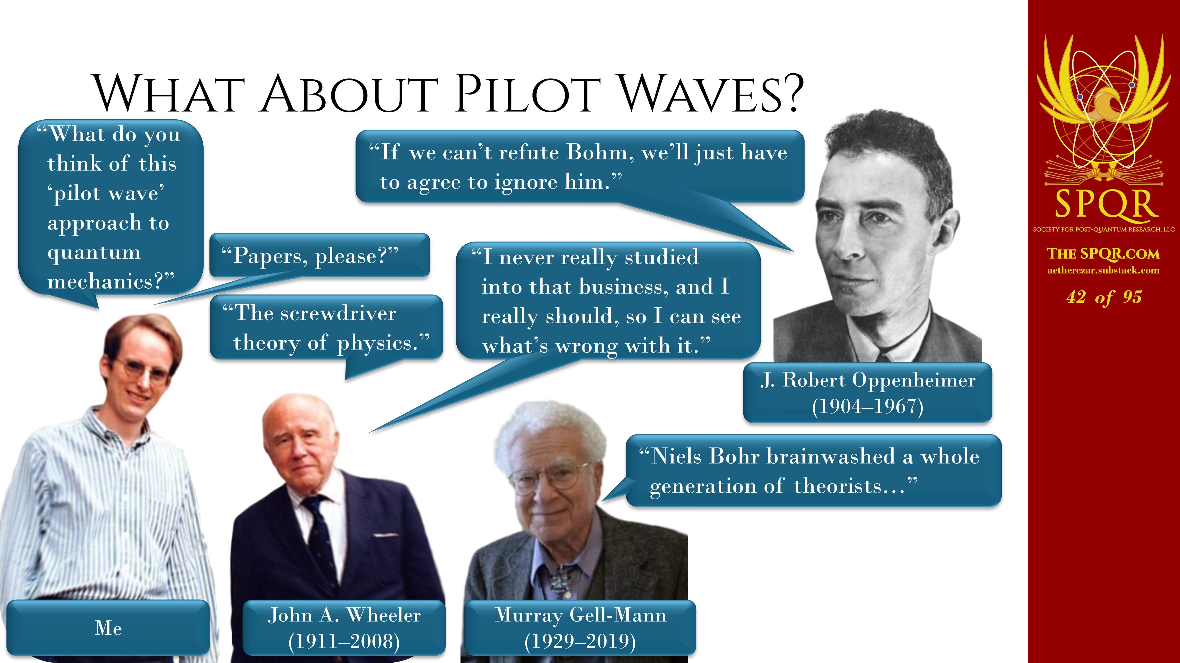
And in fact, the Nobel laureate Murray Gell-Mann commented, Niels Bohr brainwashed a whole generation of theorists into thinking that the Copenhagen Interpretation was the last word in understanding quantum mechanics.

Theory-Practice Divide

Now, there’s another issue here, not just the philosophical issues and the prejudices and blinders that people put on. There’s an issue of the theory-practice divide. I saw a wonderful example of this very recently. A hairdresser in Baltimore named Janet Stevens was in a museum looking at Roman busts. And she saw a bust like this, and she saw the little card about how this is a bust of a Roman matron wearing a wig. And she took a look at that and she said, “That’s not a wig. That’s an actual hairstyle. It’s very elaborate, but it’s an actual hairstyle.”

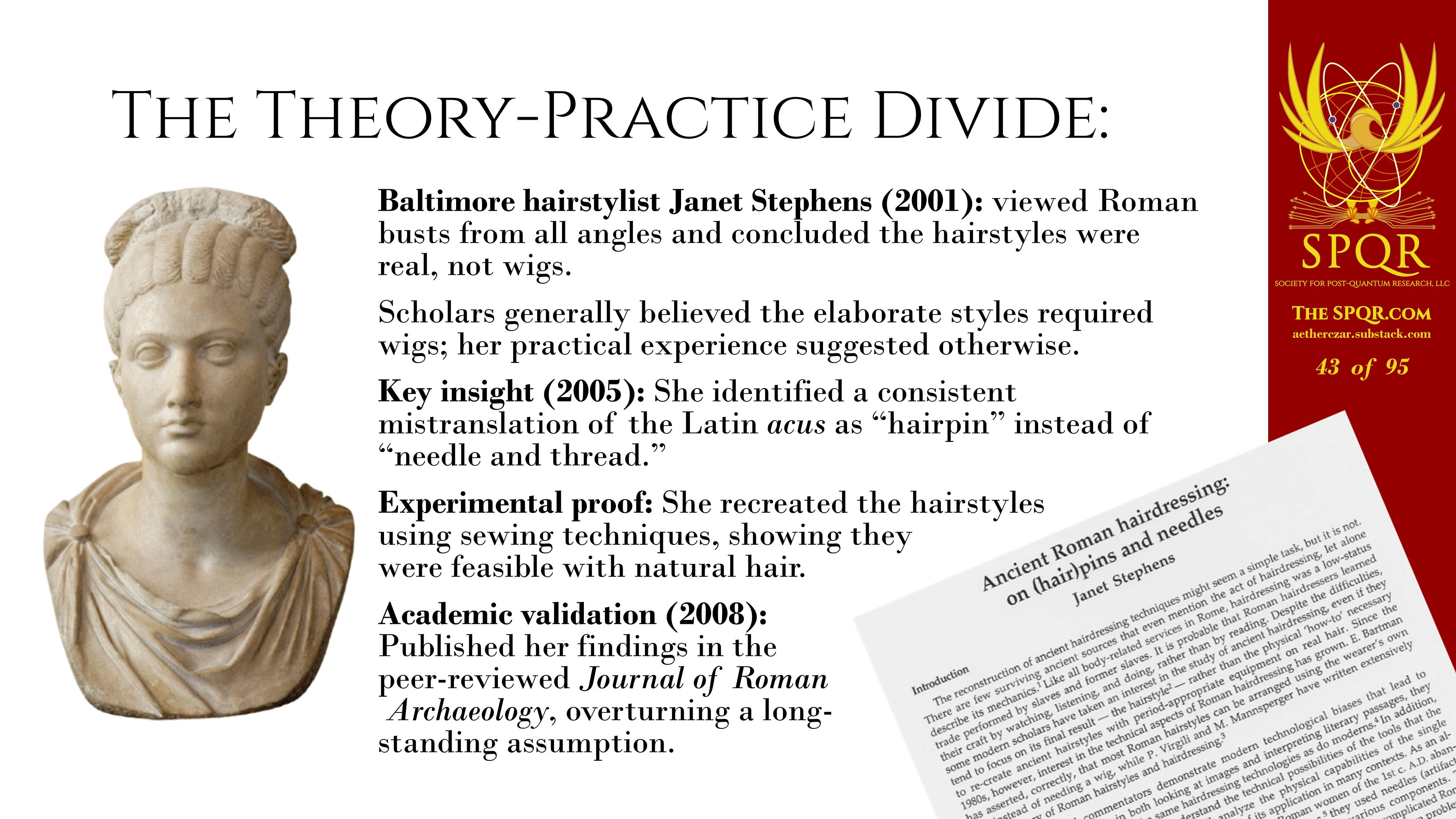
So she did a lot of research. She identified mistranslations of Latin. She recreated the hairstyles using plausible sewing techniques, showing that they could be done in a reasonable amount of time. And ultimately, she was able to validate her ideas and publish an article showing that, yes, in fact, that was an actual hairstyle and not a wig that was on the statue.

Well, that brings us back to the problem with physics. Because 80 years ago, this is the book: Electromagnetic Theory by Julius Adam Stratton. This was the bible of electromagnetism. The electrical engineers at MIT’s Rad Lab developing radar and the physicists at the Manhattan Project building the bomb: this was the book that they got their electromagnetism out of.

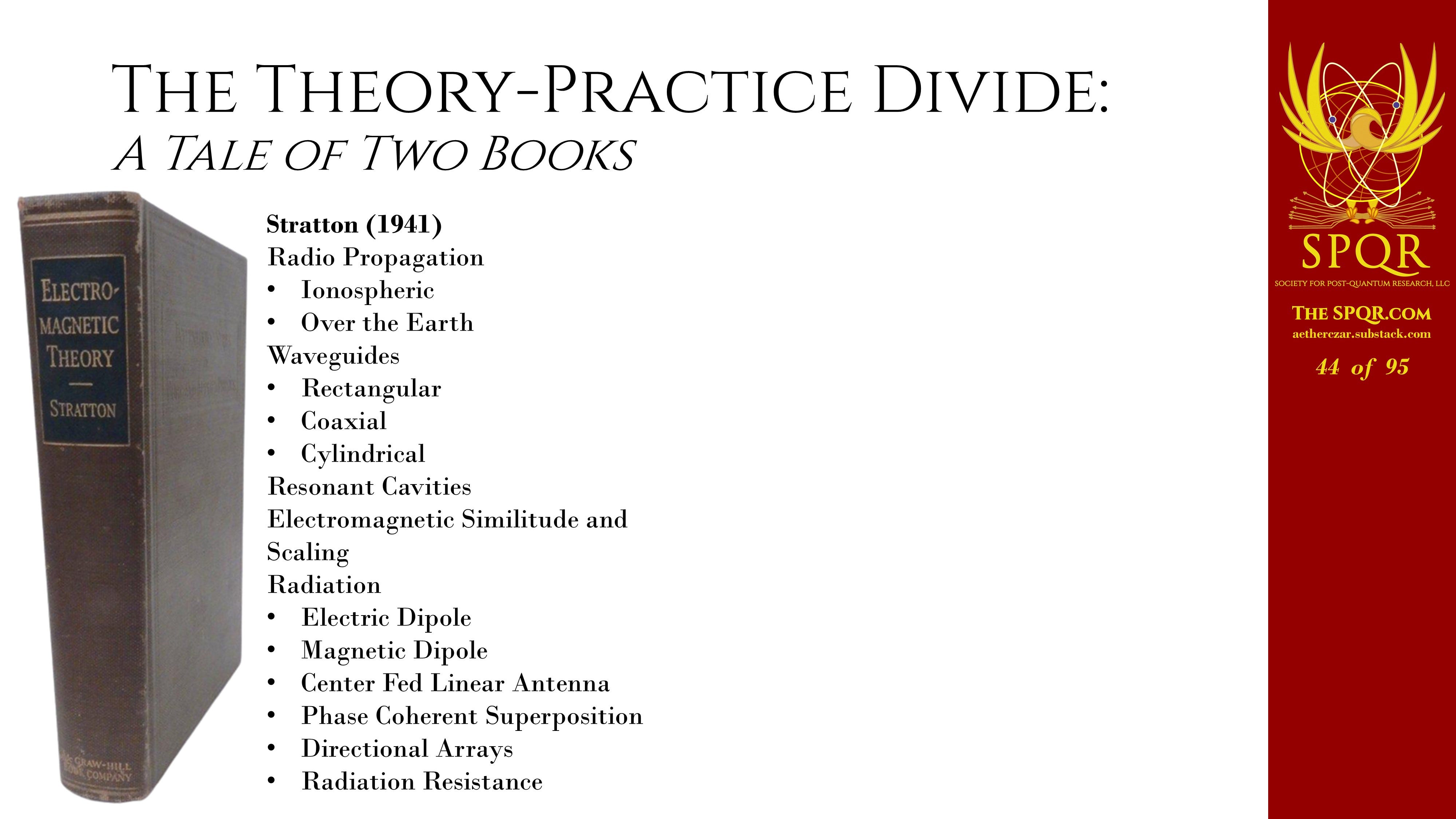
And it’s full, if you look at the table of contents, full of a lot of very practical, everyday, real world applied electromagnetic problems and considerations. Well, fast forward another 50 years or so to when I was in grad school.

And this was the book that we used. Jackson’s Classical Electrodynamics. This is a second edition. It’s a blue third edition for the youngsters taking this class nowadays.

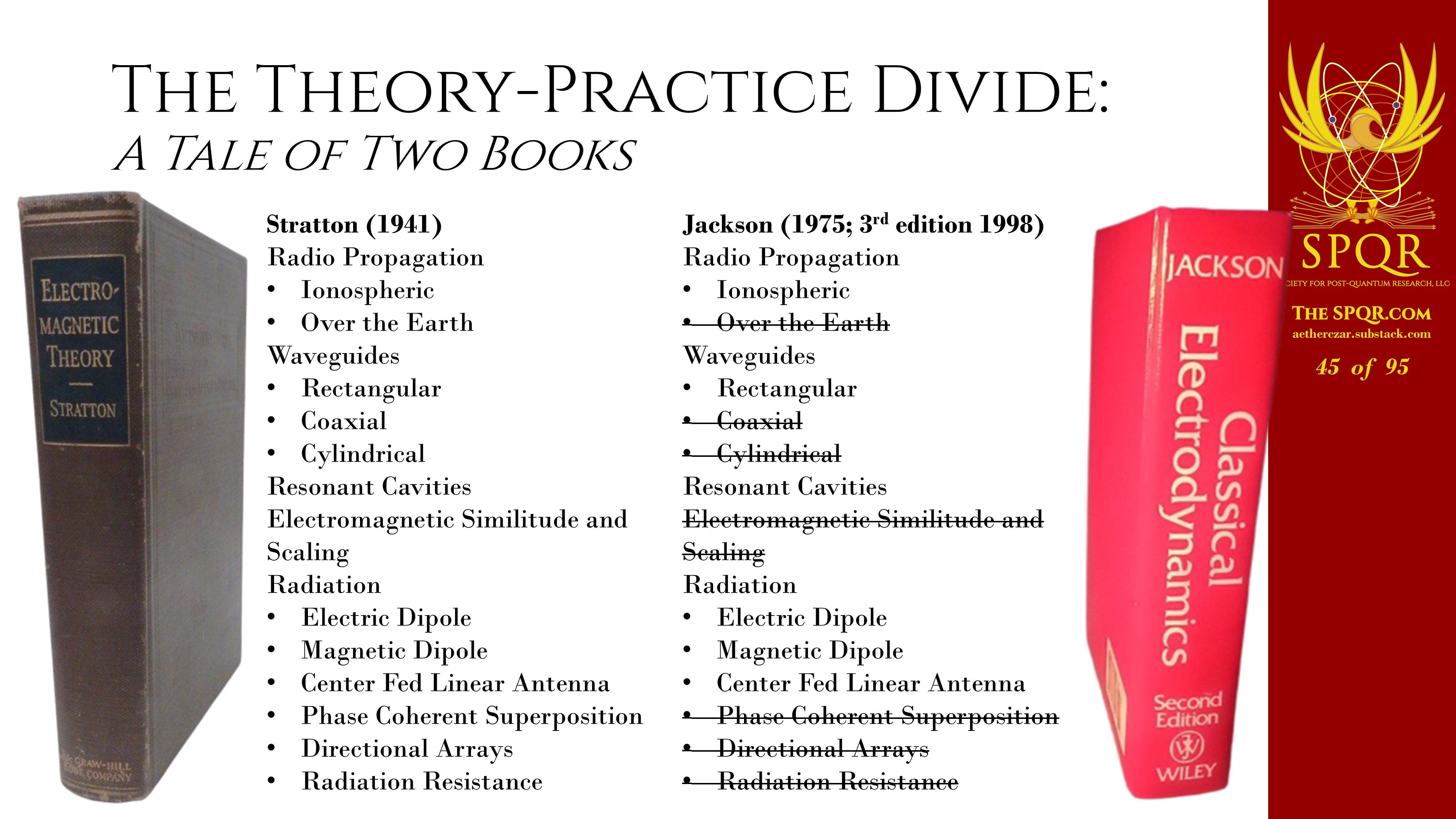
And if you do a side-by-side comparison of the applied topics in Stratton to the applied topics in Jackson, you discover that today’s physicists are taught a dumbed down and atrophied version of the applied physics that was in Stratton in 1941. And it’s worse because they don’t even bother including any of the more modern things like Smith charts and impedance matching and electrically small antenna concepts. There’s been a complete separation, a division between theory and practice.

How Fields & Energy Fix Physics

So facing that problem, what I want to talk about is how the “Fields & Energy” approach tends to fix this problem in physics.

Dirac’s Big Mistake

And I’m going to begin by going back to a train platform in Stockholm in 1933. You see here Dirac and Heisenberg and Schrodinger and two of their mothers and one of their wives standing on the platform.

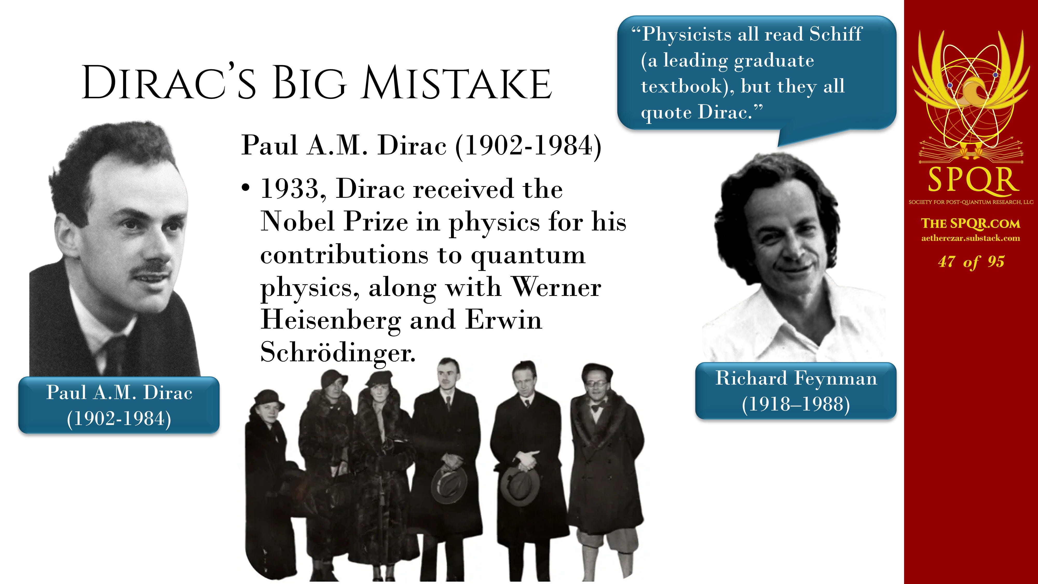
Dirac was one of the founding fathers of quantum mechanics. Feynman commented, everyone reads Schiff, the leading graduate textbook, but they quote Dirac when they want to say something important. And Dirac, in this book, his Principles of Quantum Mechanics, had a long analysis of why two photons could never, ever interfere with each other.

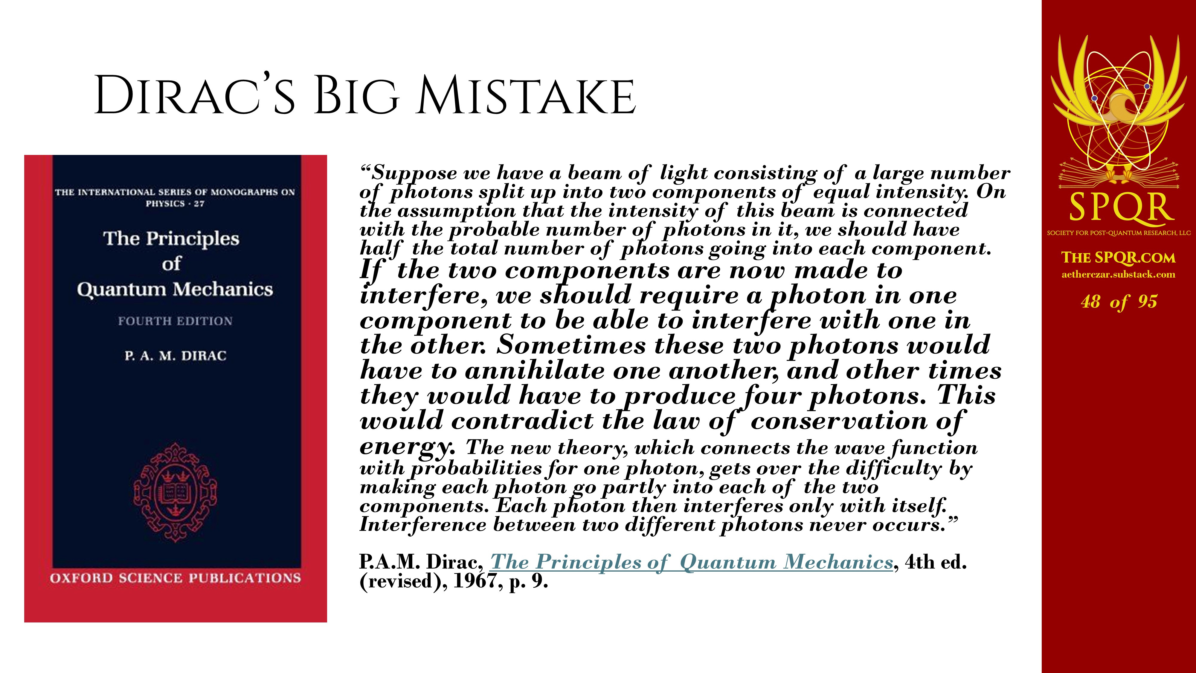
And again, I’ll spare you the wall of text. The basic idea is, he said, look, you got two photons coming together. If they add up constructively, you double the field. But the energy goes as the square of the field. So you have four times the energy. That violates conservation of energy.

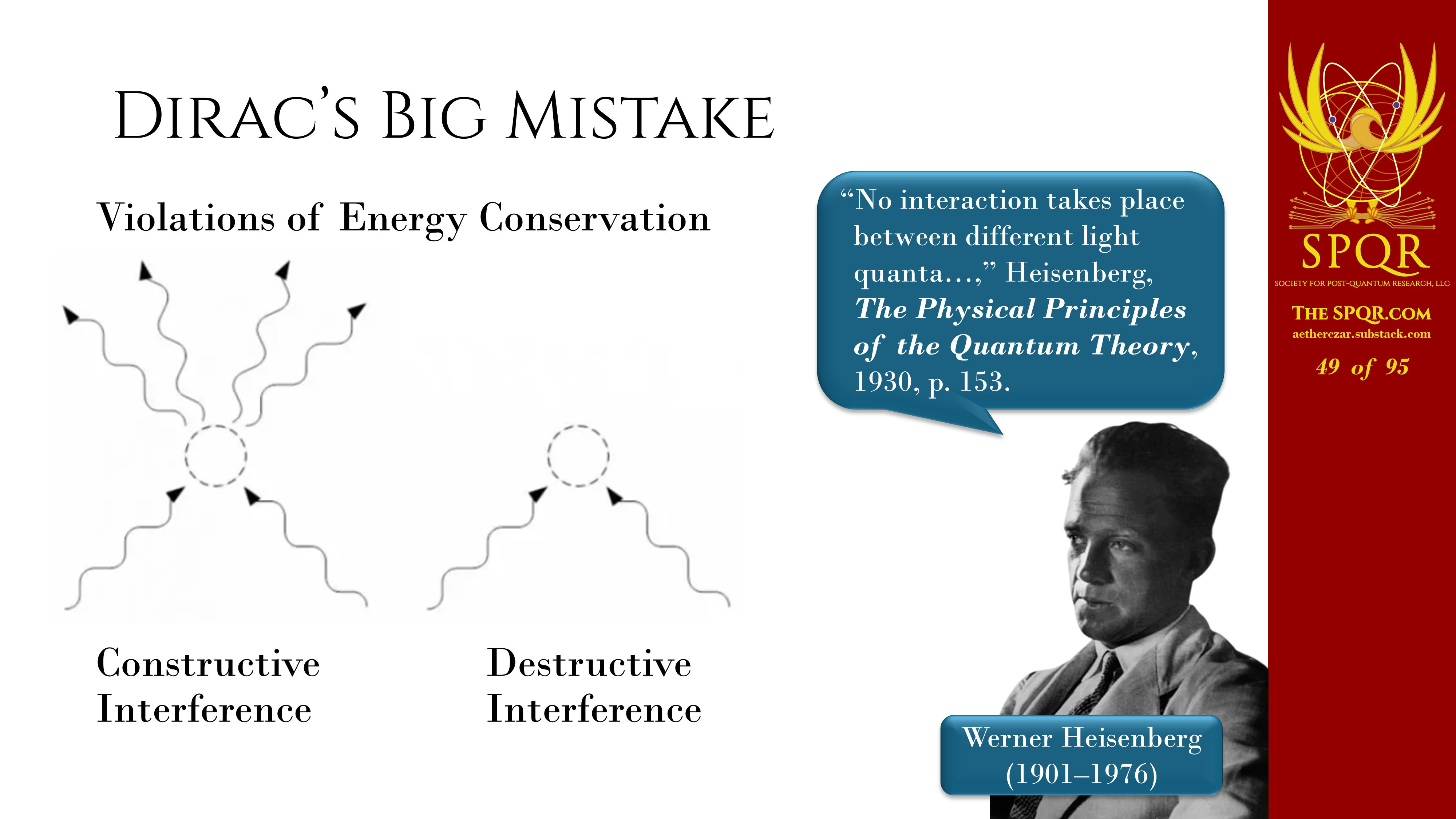
Therefore, two photons can never interfere with each other. And similarly, in a destructive interference, you’re canceling out the fields. The energy goes to zero. Again, you violate conservation of energy, so two photons can never interfere constructively or destructively with each other.

And it wasn’t just Dirac who came to that conclusion. You can see Heisenberg said more or less the same thing in his textbook in 1930.

How Electromagnetic Waves REALLY Interfere

Well, let’s take a look at that and use some of our basic right-hand rule, electricity and magnetism, if we can remember that from our undergraduate days, and consider a small forward wave and a small reverse wave in constructive interference.

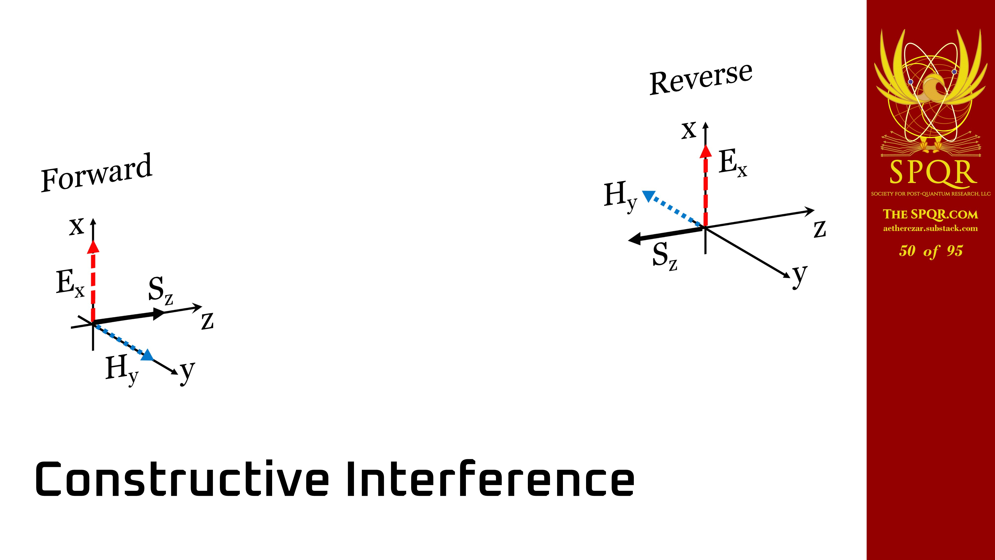
Of course, we define interference with respect to the electric field. When they come together, yes, we’re going to get twice the field, and we’re going to have four times the electric energy.

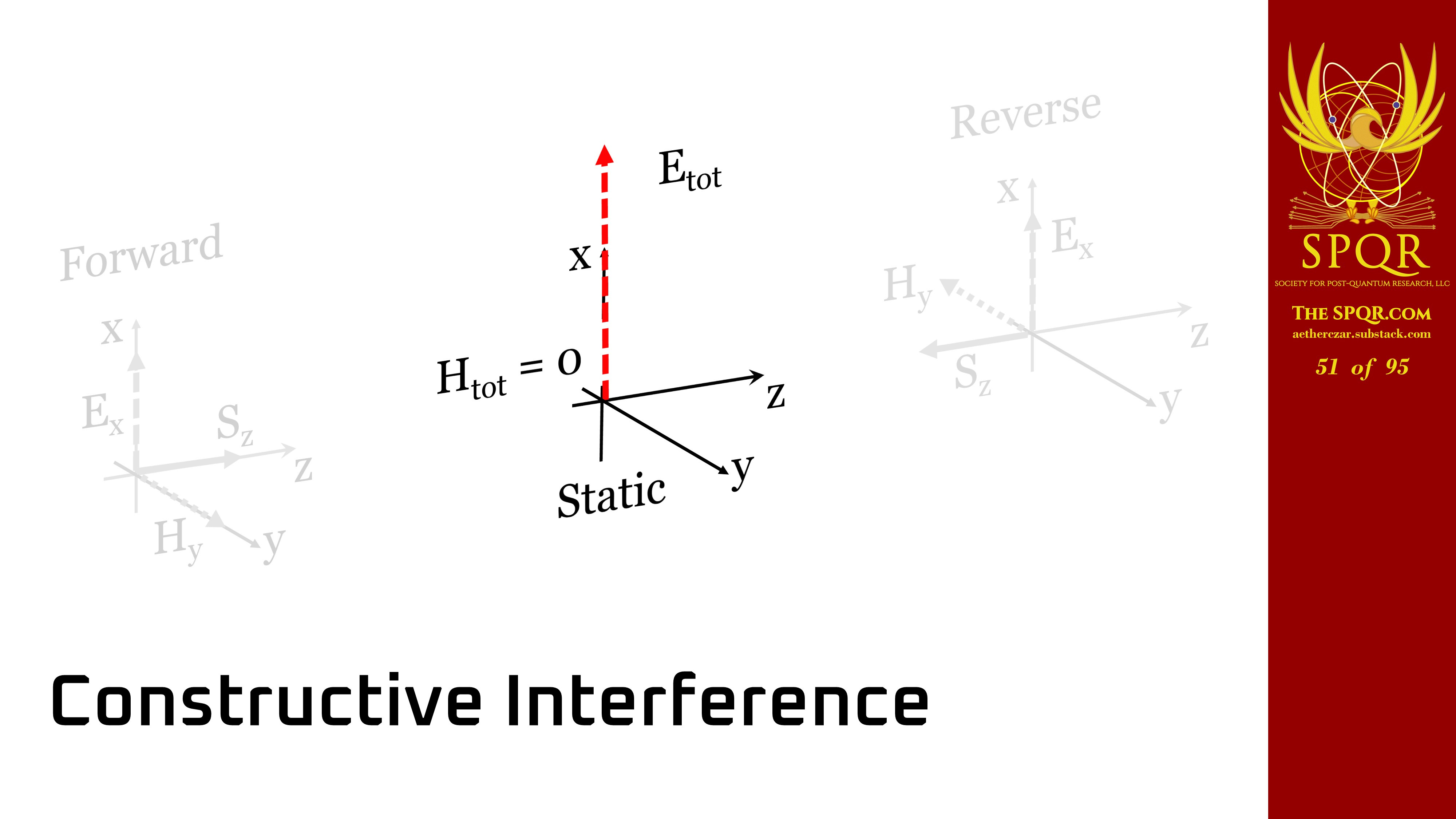
But notice what happened to the magnetic field. When we reinforce the electric field, we are canceling out the magnetic field. And remember, going back to Heaviside’s great discovery, there is a balance of electric and magnetic energy in the wave. So what’s happened is we’ve canceled out the magnetic field. All of that original magnetic energy has become electric energy. So energy conservation is satisfied. It’s just a transformation of the original balance of electric and magnetic energy in the moving wave to purely electrostatic when we have a constructive interference.

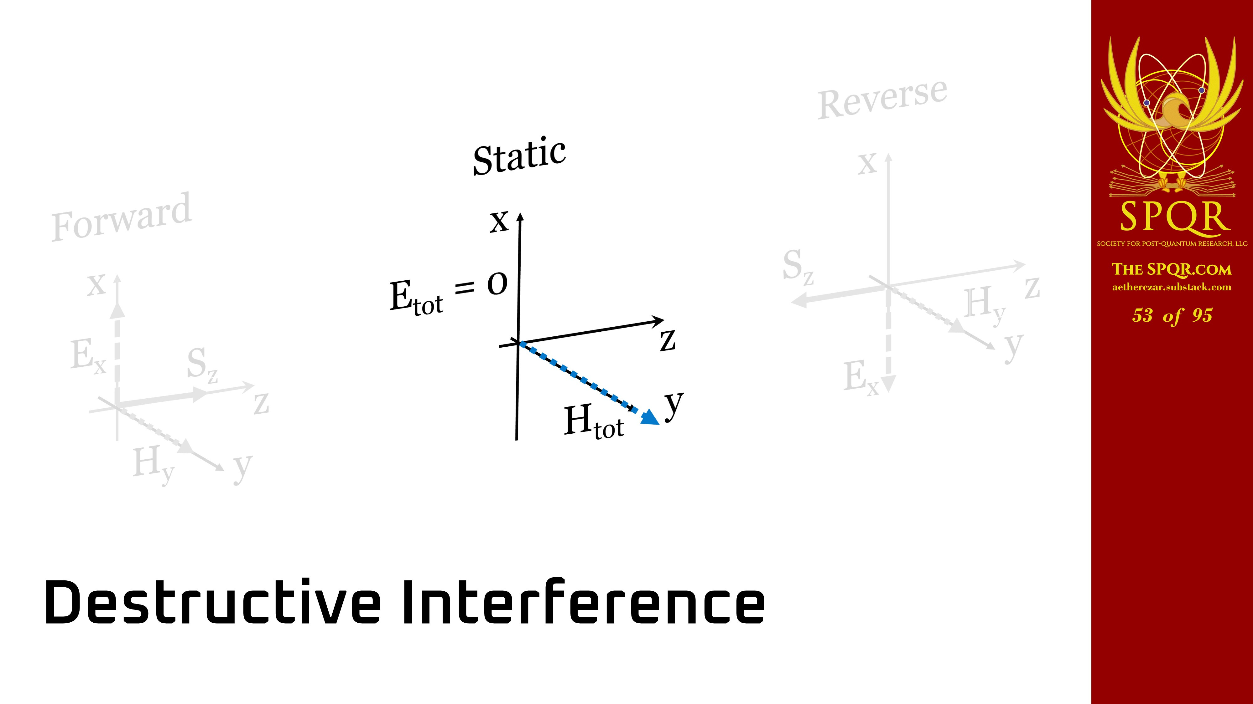
And similarly, if we look at a destructive interference, yes, the electric fields are going to cancel out.

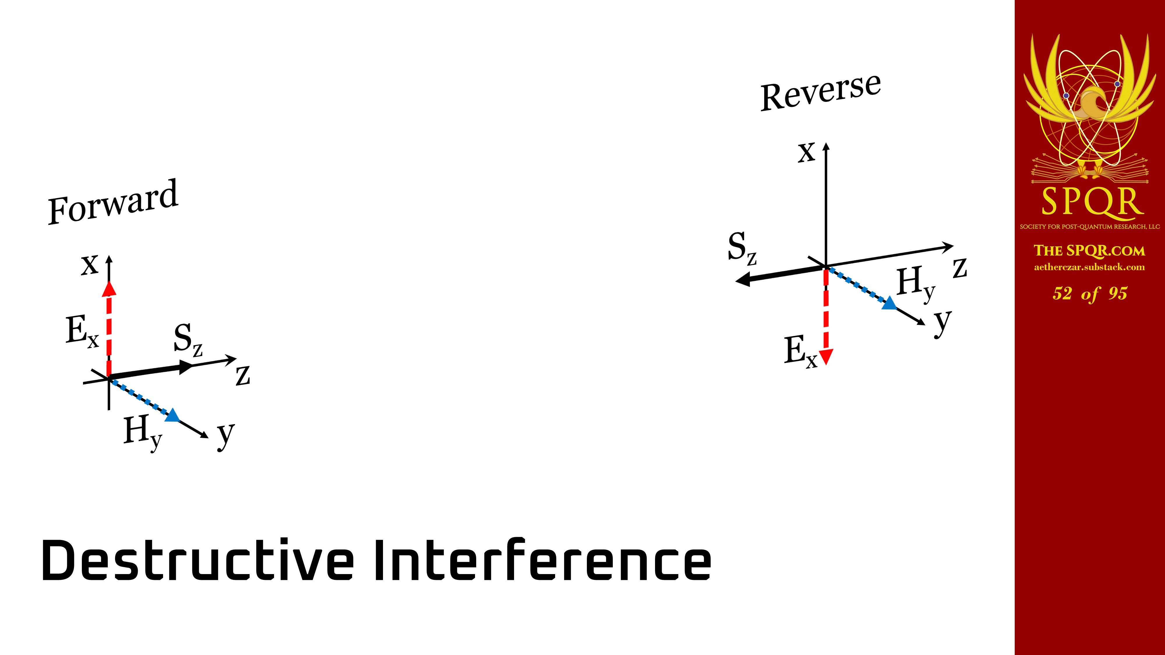
But look what happens to the magnetic fields. They double, they reinforce, that balance has shifted to be all entirely magnetic energy.

Now, I have to put some equations in here or they’ll revoke my PhD.

The Great Circle of Electromagnetism

But what I want you to note here is how you can use microwave impedance electrical engineering type approaches to the problem to understand this in a very simple way.

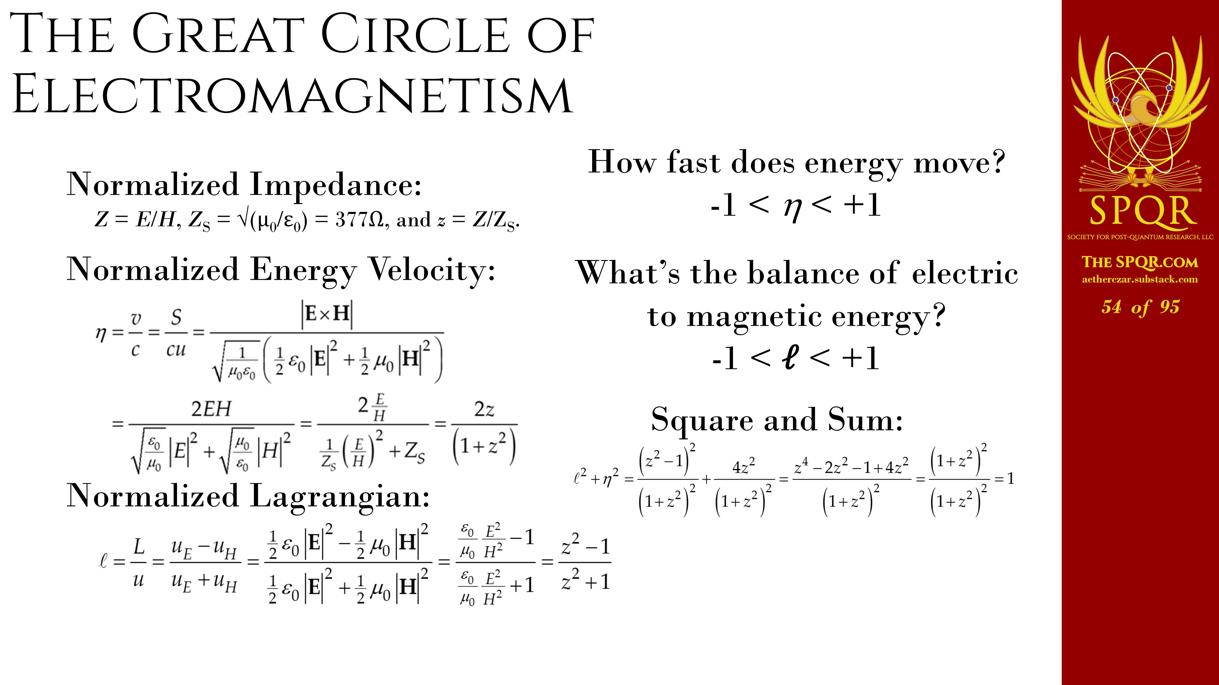
If you take the energy velocity that was pioneered by Heaviside and take a parameter that physicists use called the Lagrangian. The Lagrangian is basically the difference in the electric versus the magnetic energy. We normalize the energy velocity with respect to the speed of light, and we normalize the Lagrangian with respect to the energy density. That gives us two parameters. The normalized energy velocity goes from minus one to plus one, moving backwards or forwards at the speed of light, and zero would be stationary. The normalized Lagrangian tells us the balance of electric to magnetic energy. Plus one would be all electric, zero would be a balance, and minus one would be all magnetic.

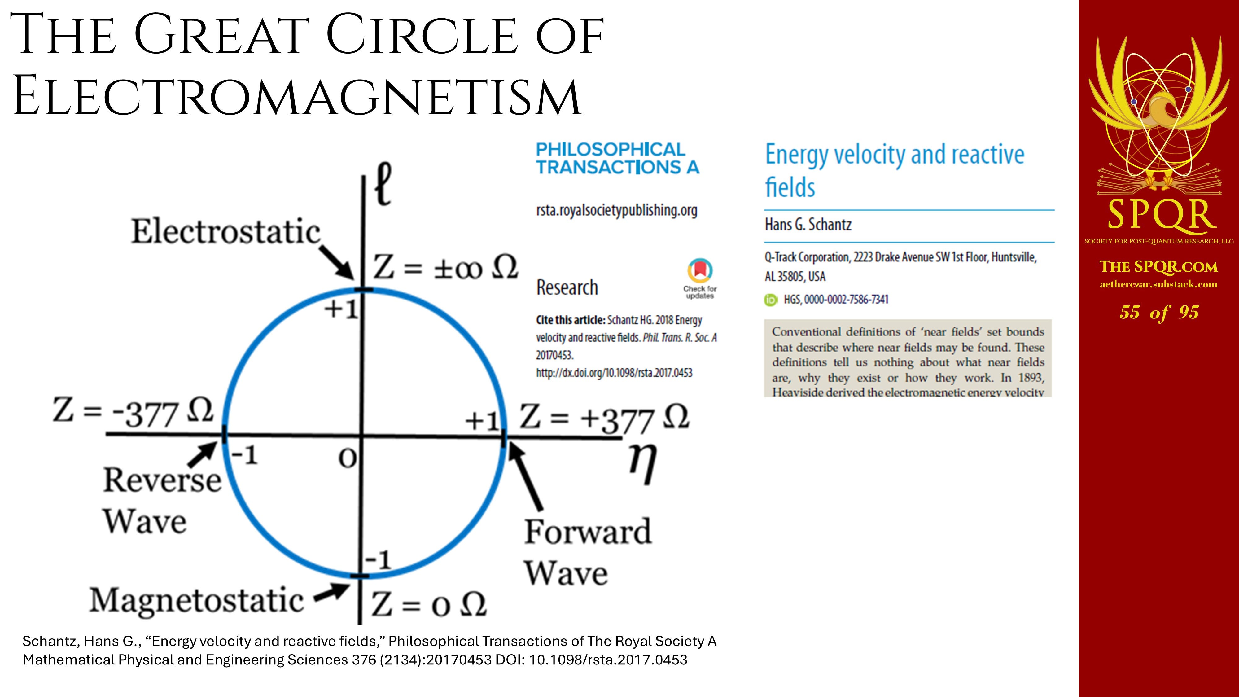
The fascinating thing is, if we square and sum those two quantities, ell squared plus eta squared, it’s equal to one. And that is the equation of a unit circle. So this unit circle describes how a 1D wave will work. We start with a forward wave. If we come to an open, say, the energy becomes all electrostatic, turns around and goes in the opposite direction. In the reflection, we have the reverse wave.

Or if it interacts with a short, it goes the other way around the circle. It becomes purely magnetostatic and then becomes a reverse wave. And you can see all of this math is in my paper, “Energy, Velocity, and Reactive Fields,” if you want to go into it in more detail.

But of course, this should raise an immediate question, wait a moment, electrostatic and magnetostatic?

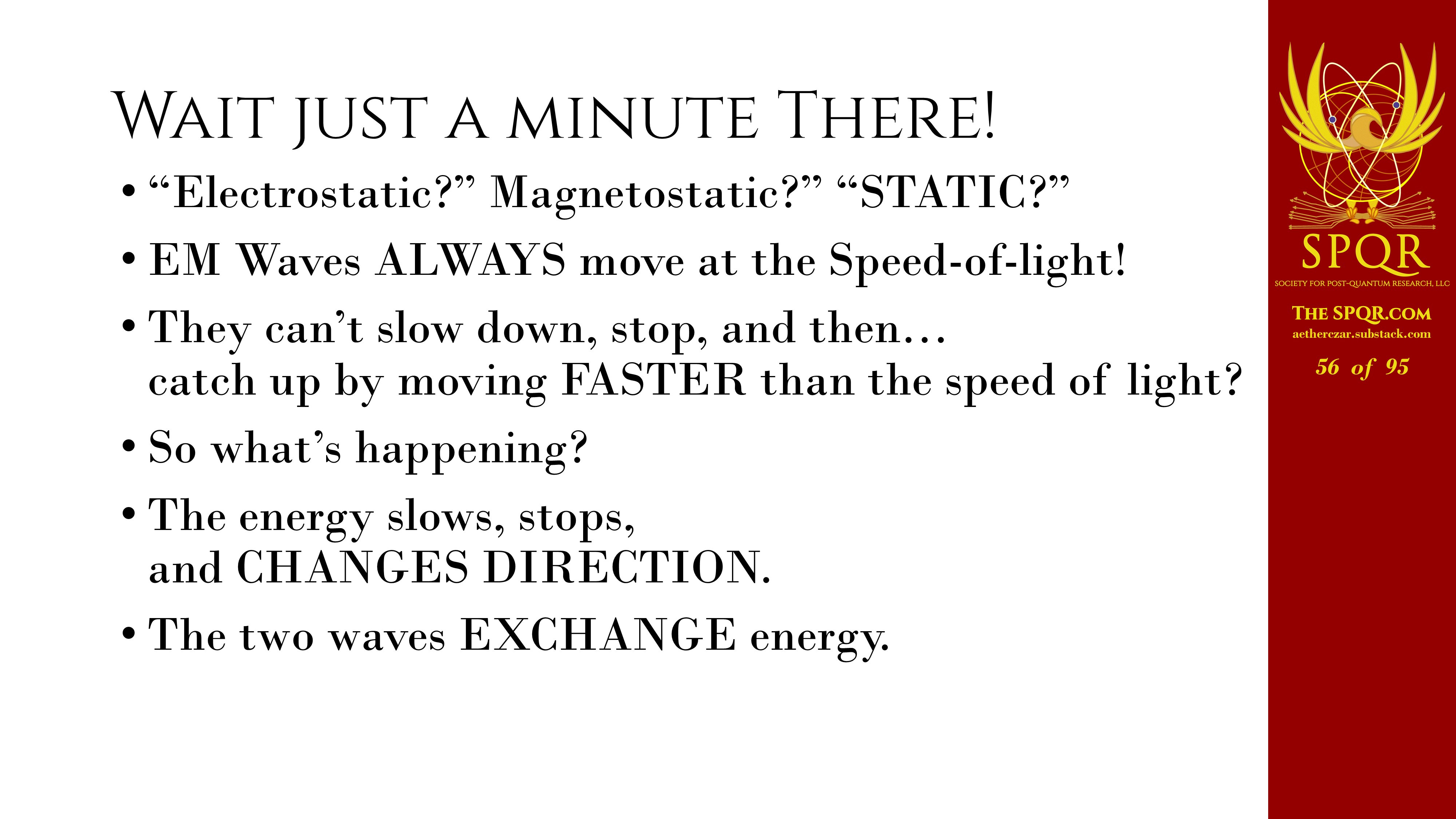
Static… we’re talking about energy not moving, being associated with fields that are moving at the speed of light. How can that be? Well, the reason is that the energy is slowing, stopping, and changing direction. The fields, when they interact with each other, are exchanging energy with each other.

How Electromagnetic Waves Interact

So we start with two waves moving down a transmission line, mirror image waves. The axes are scaled, so the speed of light is at a 45-degree angle.

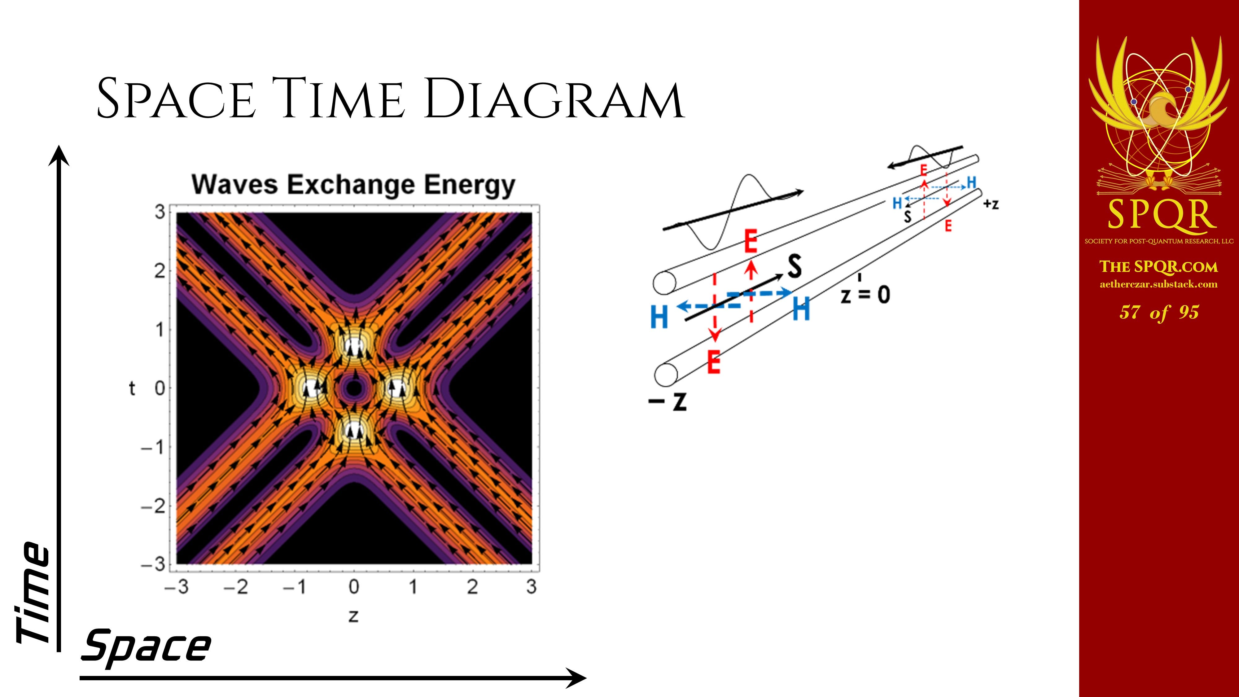
We end up with the two lobes of the forward wave interacting. We’re interacting with the two lobes of the reverse wave. Initially, the two goes-up lobes align and we get an electrostatic node.

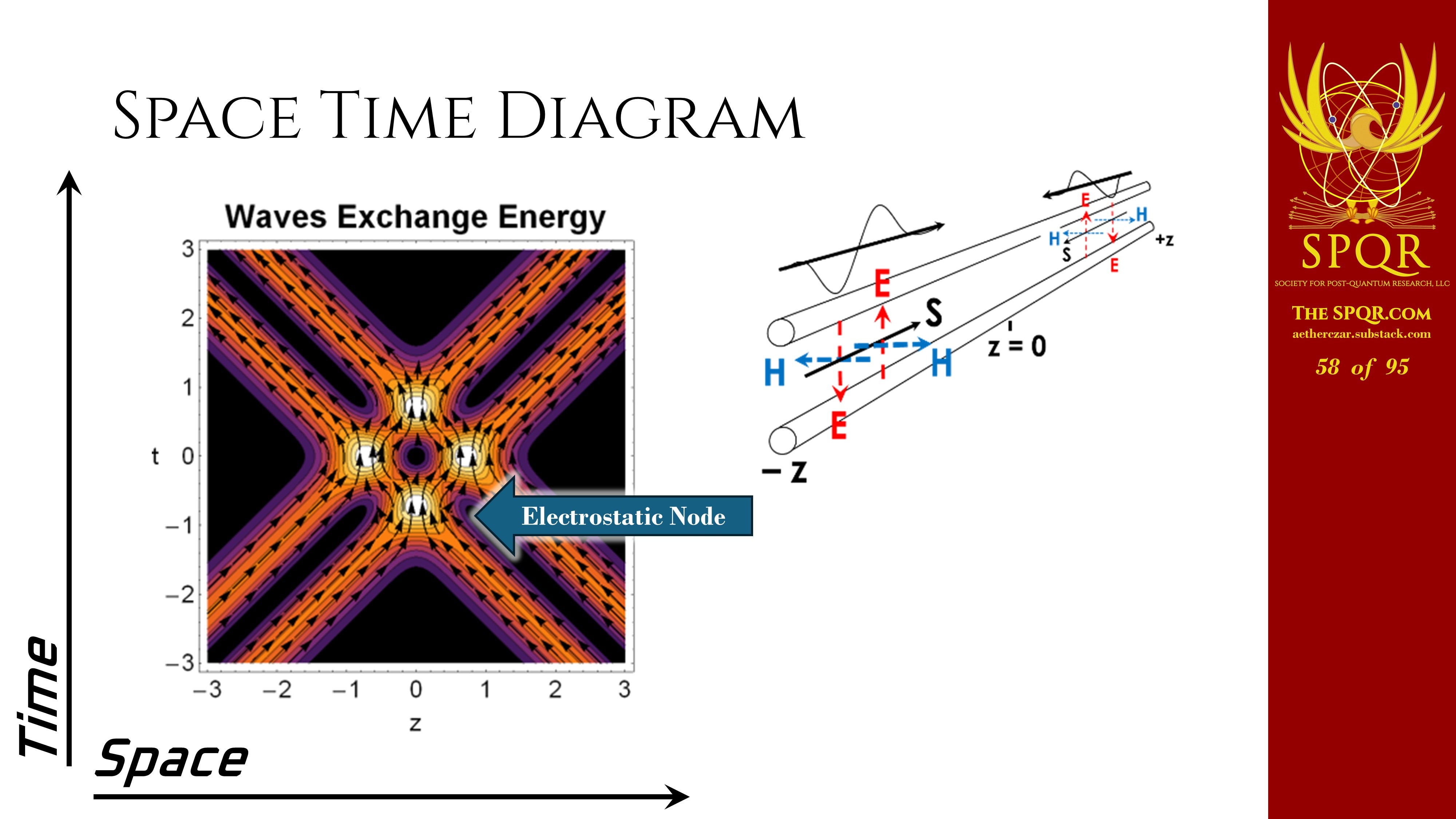
As the waves are perfectly aligned, they cancel out and we have two magnetostatic nodes.

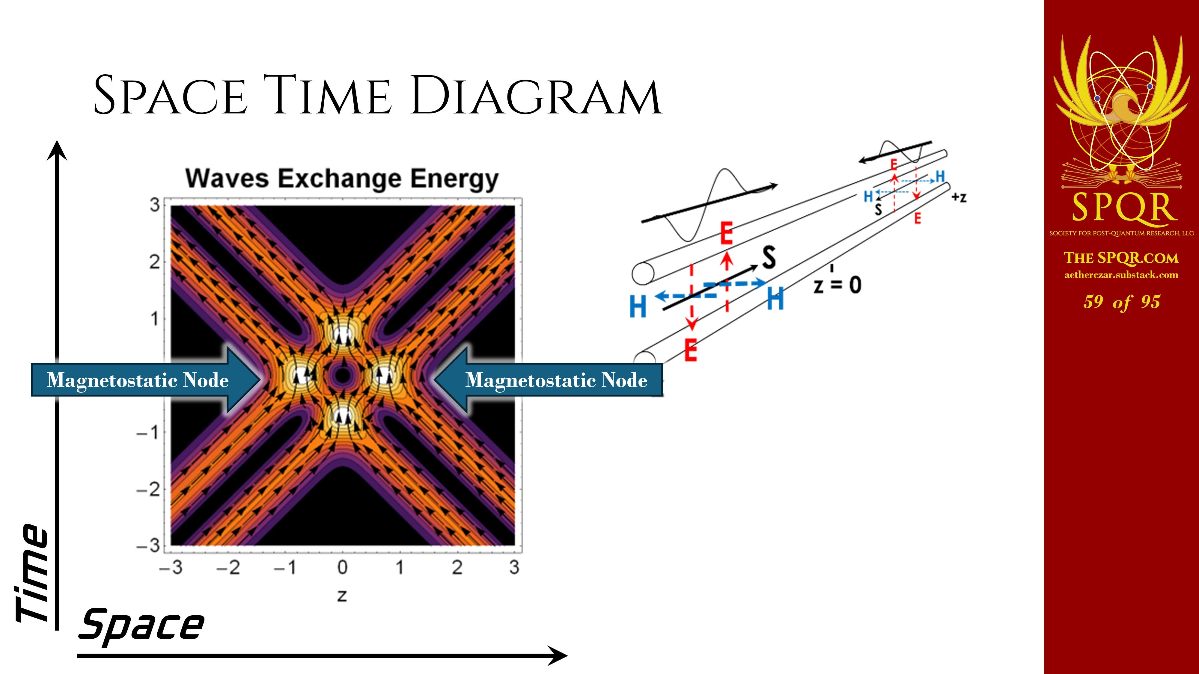
And then as they begin to separate, the two goes-down lobes add up and we get an electrostatic node.

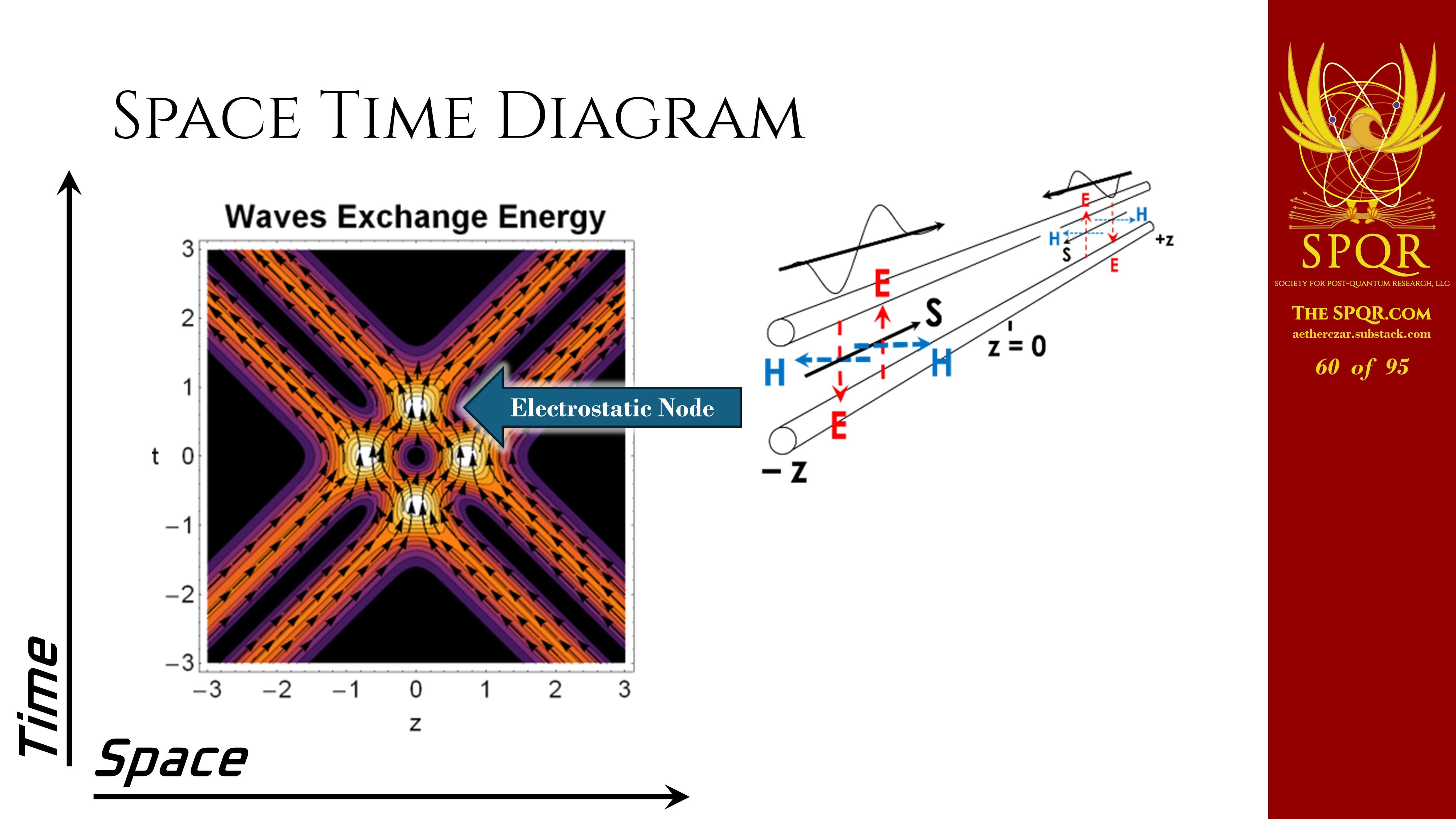
The two waves pass through each other at the speed of light, but the energy bounces. It’s exchanged from one wave to another through these interferences.

How Sine Waves Interact

We can look at sine waves the same way.

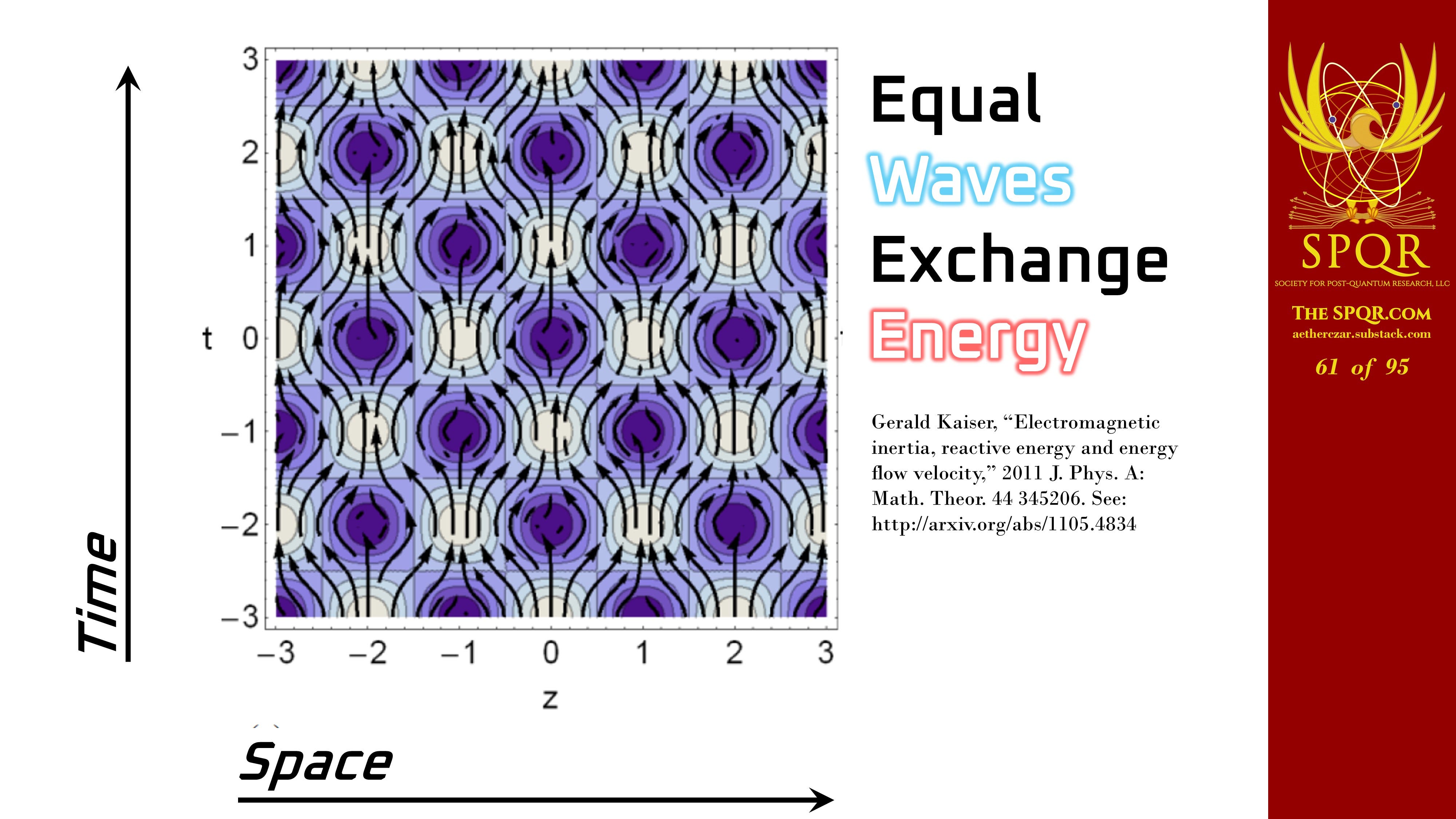
If you take a look at a forward wave moving at the speed of light…

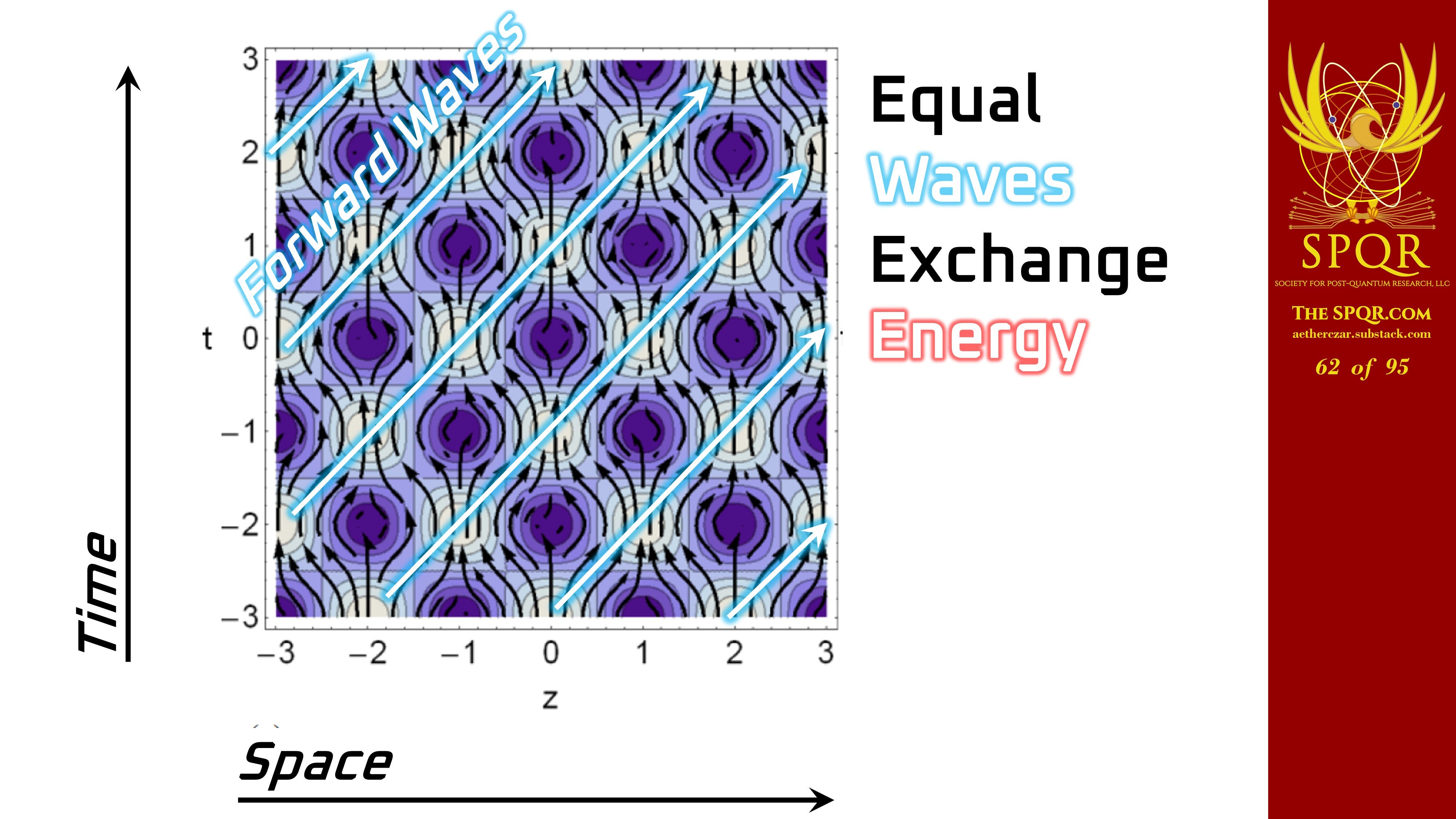
…and an equal and opposite reverse wave moving at the speed of light. If the VSWR is infinite, if you’re hooked to an open or a short, you get an equal and opposite reverse wave.

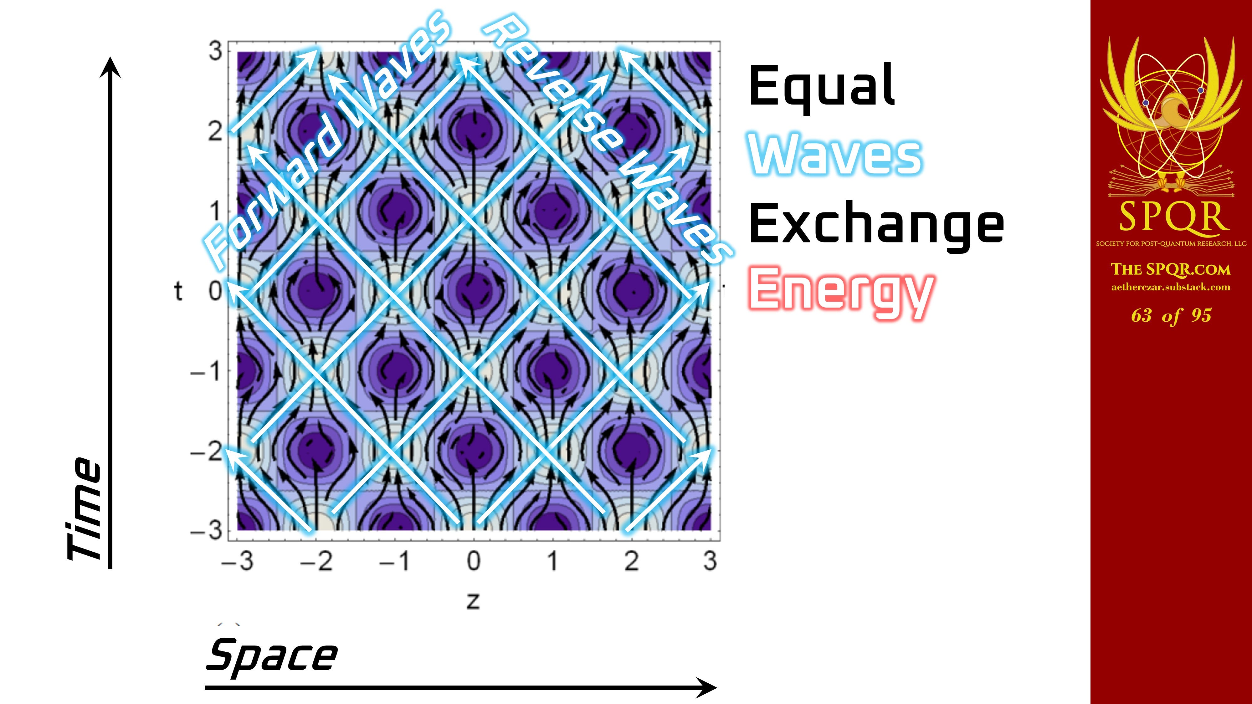
What you discover is the energy is oscillating every quarter period, a quarter wavelength between electrostatic and magnetostatic nulls.

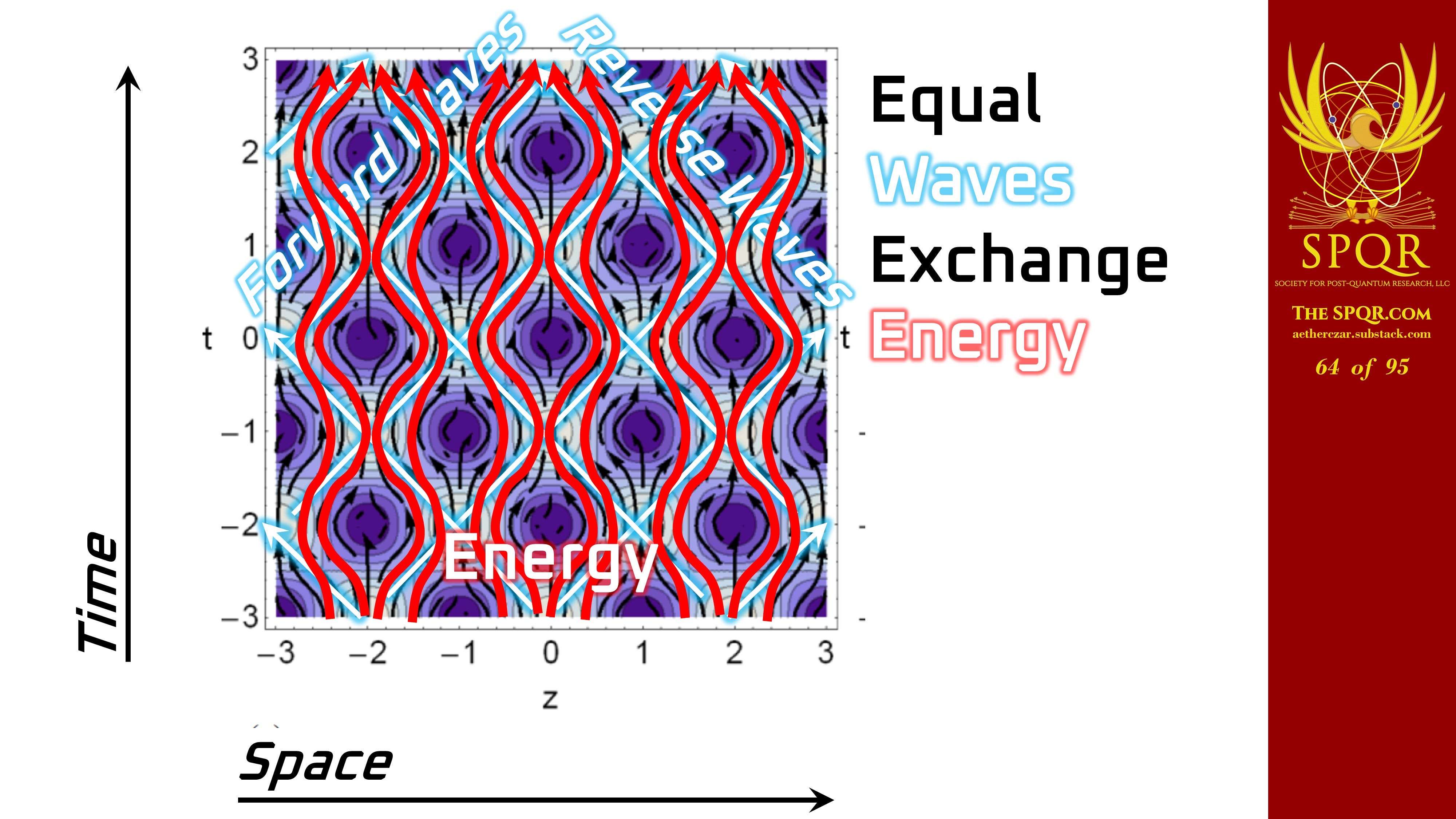
So we have the waves moving at the speed of light and the energy oscillating a quarter wavelength one way or the other.

Different phenomenon, different behavior.

We can make one wave a little bigger…

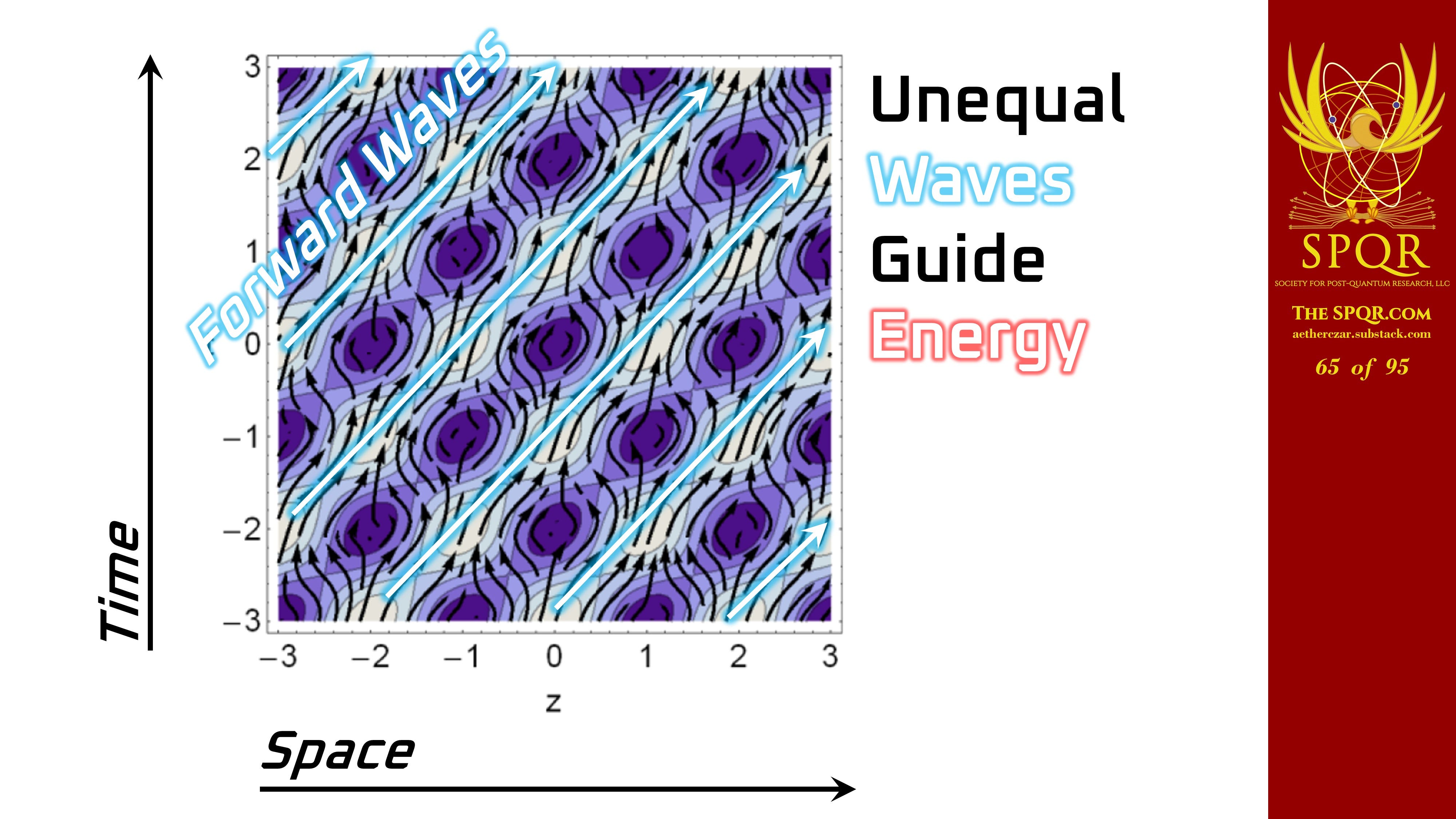
…than the other…

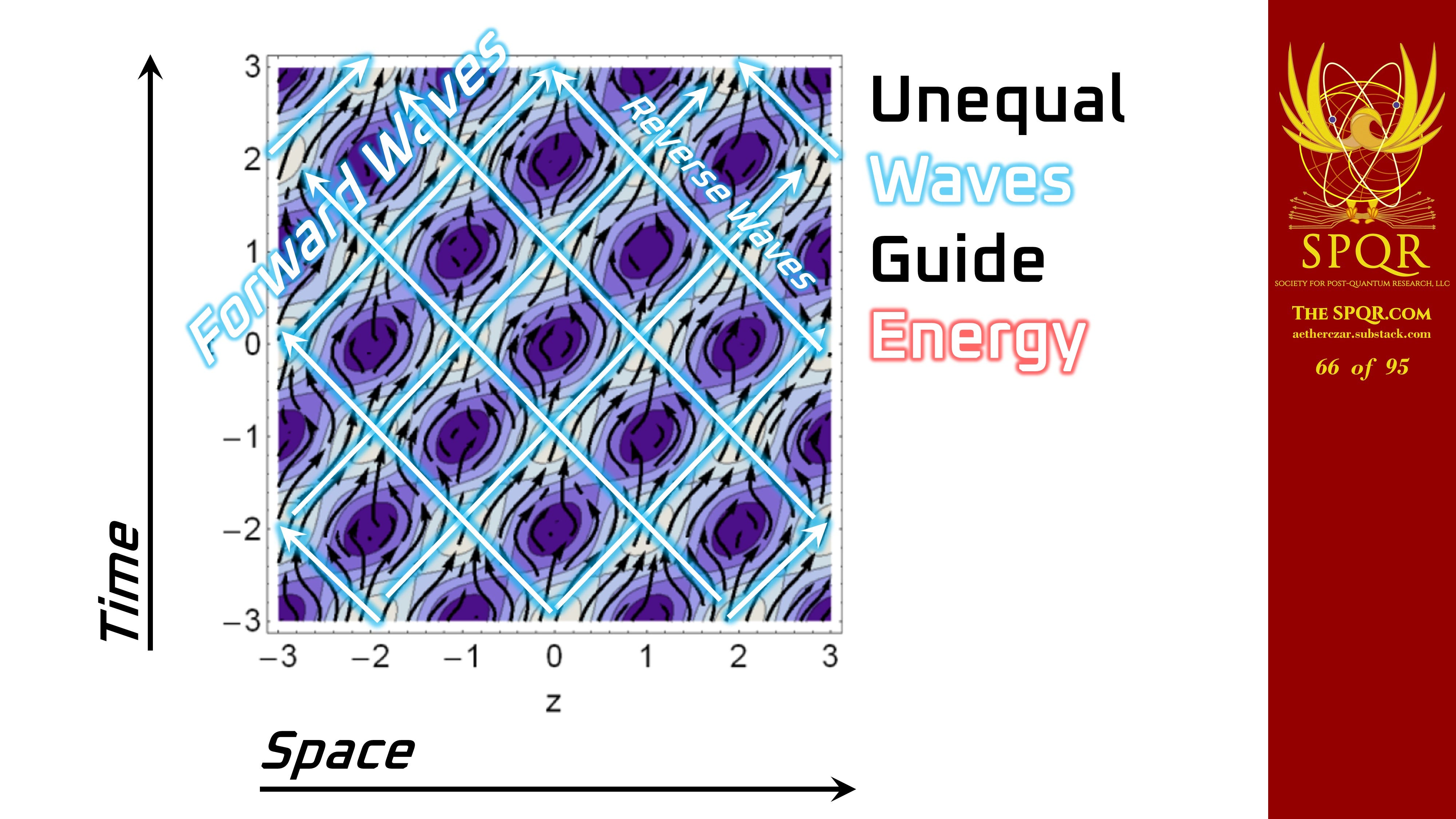
and we’ll see a little bit of a net forward progression.

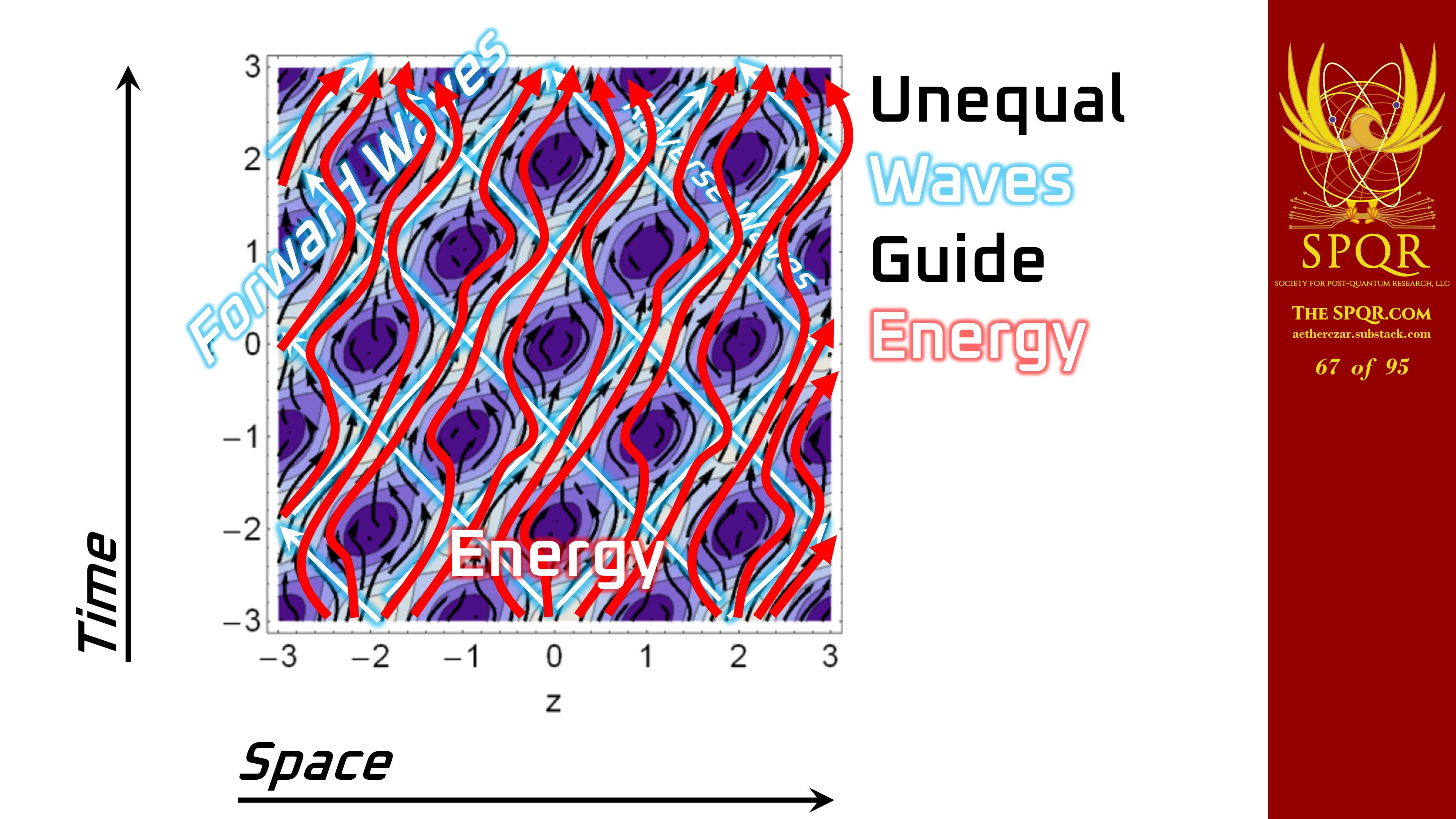
The larger forward wave dominates the reverse wave. We get a little bit of energy flow in the forward direction, but it’s at a speed that’s slower than the speed of light.

So again, different paths, different space-time behaviors.

How Antennas Work

If we look at the radiation of an antenna, we have from a small dipole energy oscillating in and out.

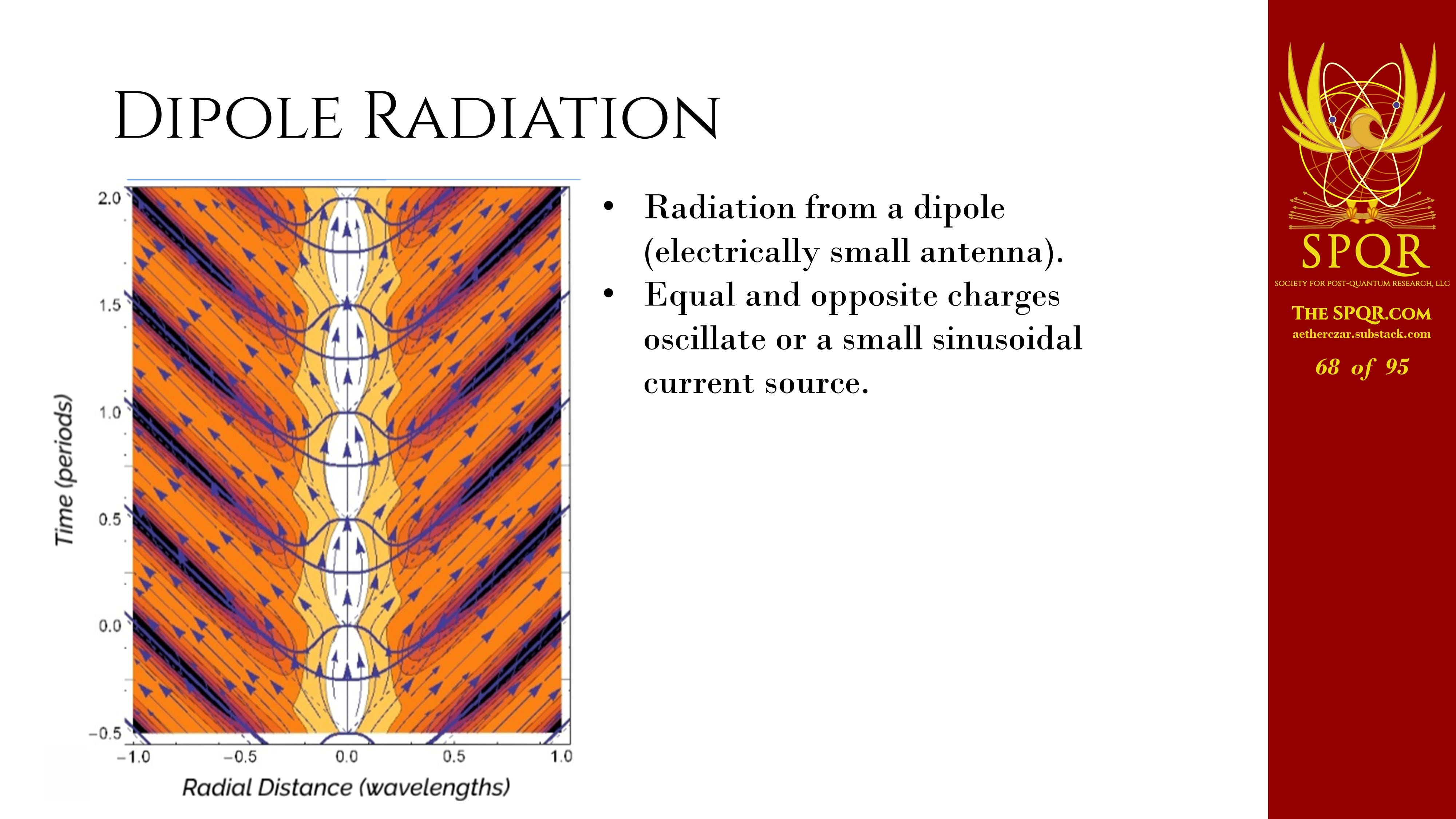
Each oscillation, when we have a field that radiates away at a given point…

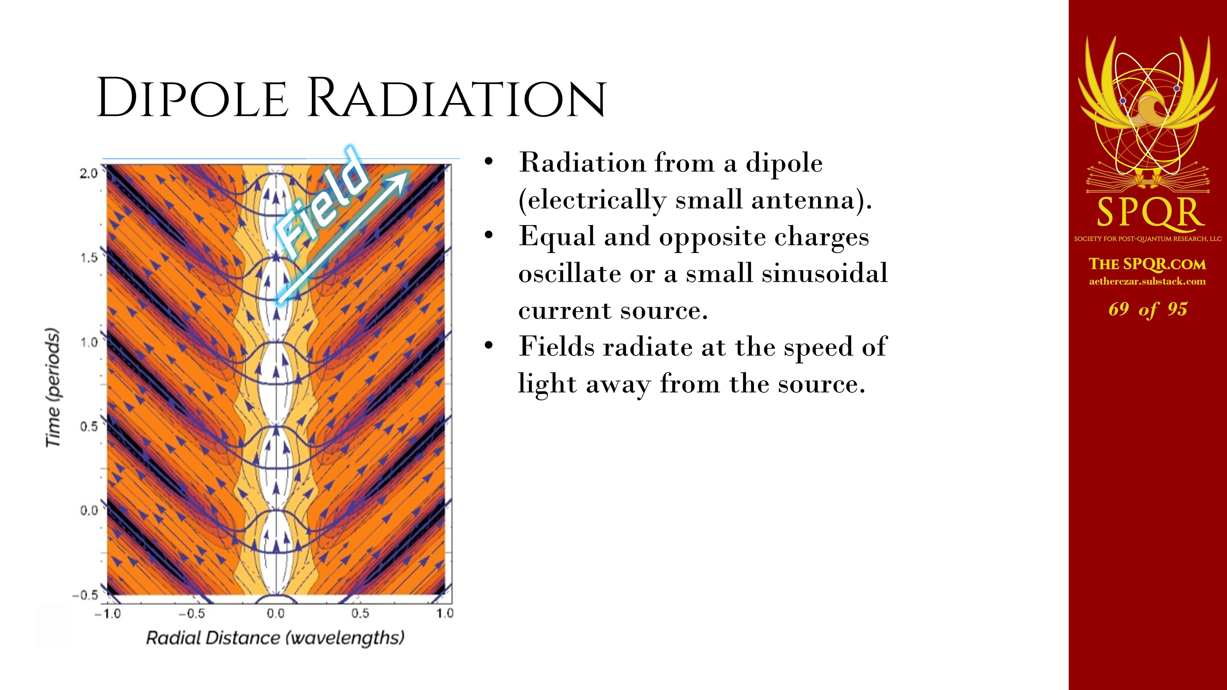
…the energy associated with it started close to that dipole.

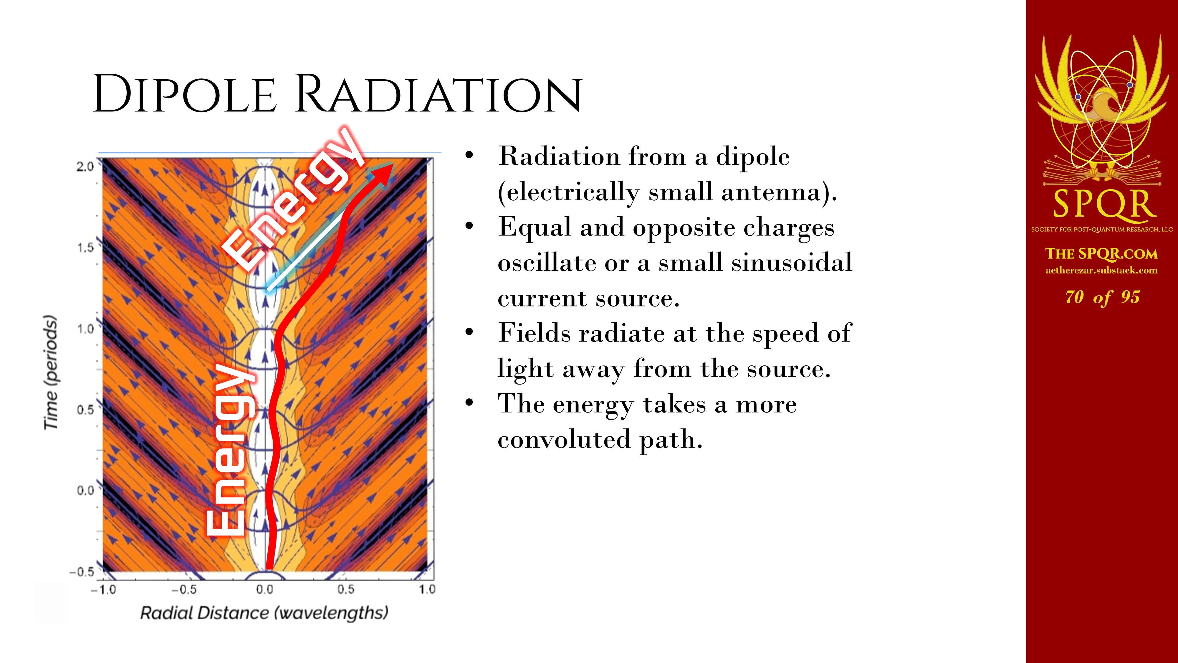
And with each oscillation, it gets pushed to another layer of the onion of energy around that dipole until finally it’s in the outermost layer and it couples to a field and gets radiated away into the far field.

Right-Hand Rule for Radiation

We can take a look at a right-hand rule for radiation. And I’m amazed that this isn’t something that I was taught, say, as a freshman studying physics. We’re all familiar with the current going in the direction of our thumb and the induction field in the direction of our fingers. That’s the IEEE logo that’s out there in the hallway.

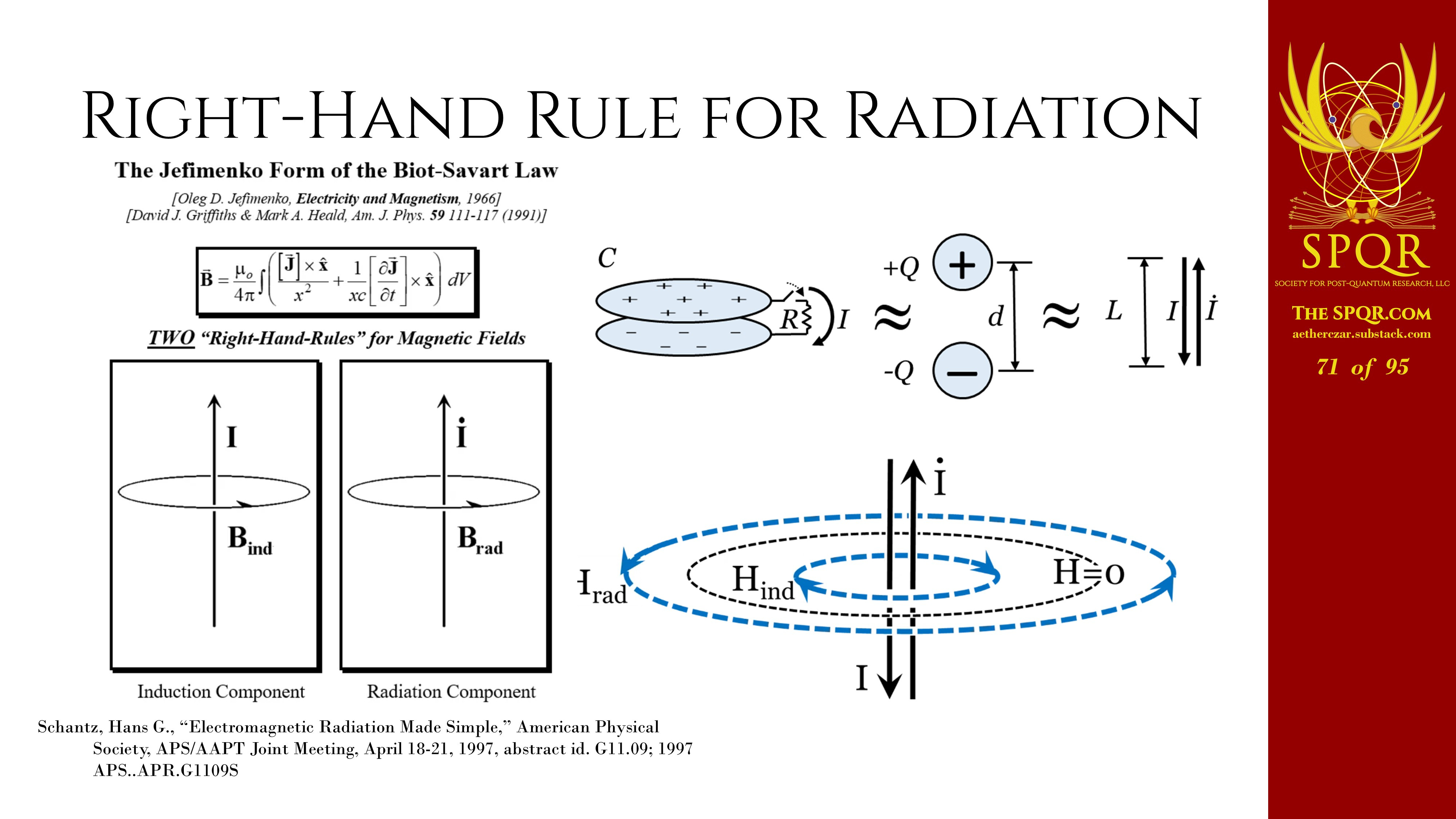
But it’s the same geometry for the radiation component of the magnetic field if we put our thumb in the direction that the current is changing. So for instance, if we have an exponential decay, We make a capacitor and we discharge it through a resistor. We have a current going down, giving us an induction field, and that current is decaying, so the I dot is in the opposite direction, giving us a radiation field. Somewhere in between there, there’s a circle where the magnetic field has to go to zero.

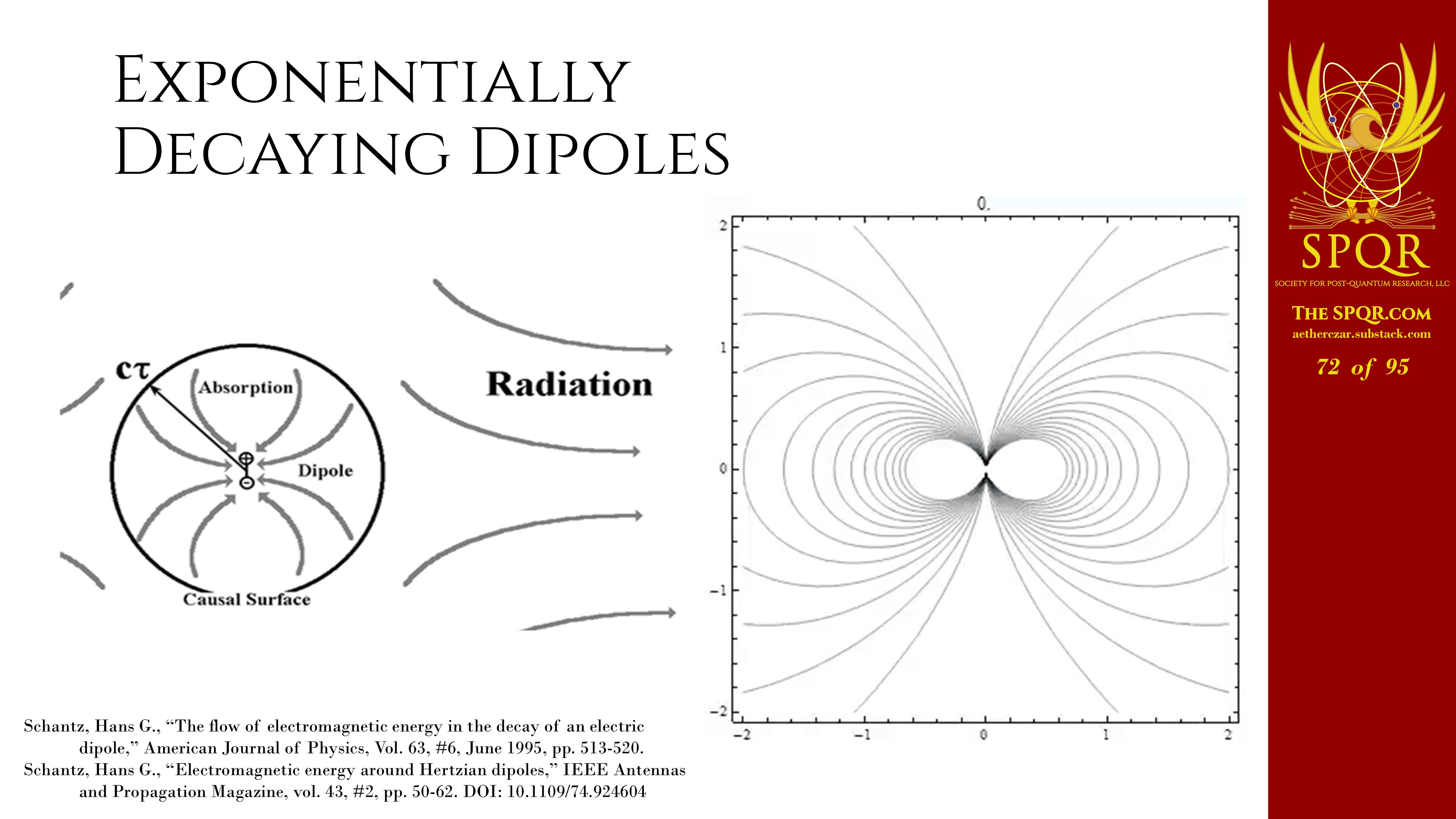
There is a bubble around this exponential decay, a bubble whose radius is the speed of light times the time constant, where the magnetic field goes to zero. No energy passes through that sphere.

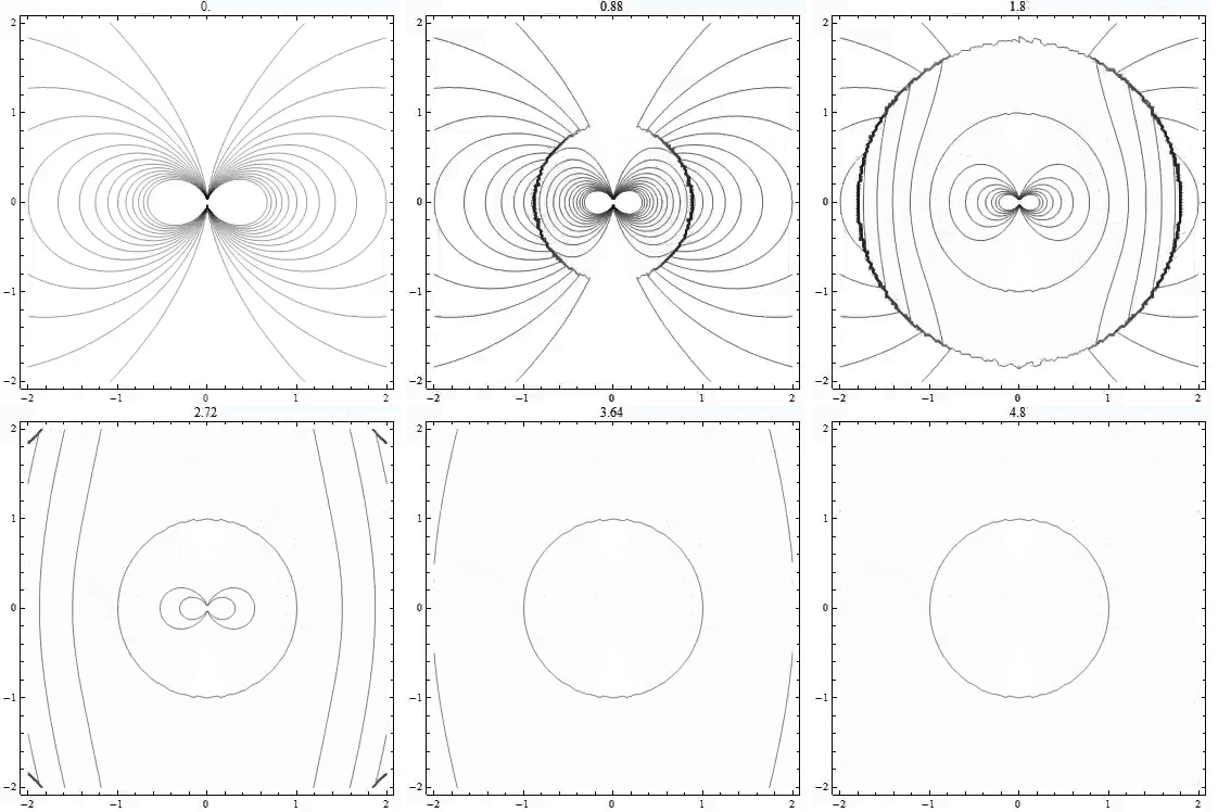
And in fact, if you take a look, at the total integrated radiation power that comes off of that exponential decay, it is exactly equal to the static field energy that was stored outside that bubble. So the radiation fields are propagating out through the inward flux of energy through that bubble. They couple to the static field energy and radiate away.

Another example that’s tough to explain, from the “single charge radiating” model…

If you take two orthogonal antennas and feed them in quadrature, this is something antenna engineers do to create a quasi-isotropic antenna pattern. And if you study the energy flow, If you find it comes off on a tangent line lambda over pi away from the source itself.

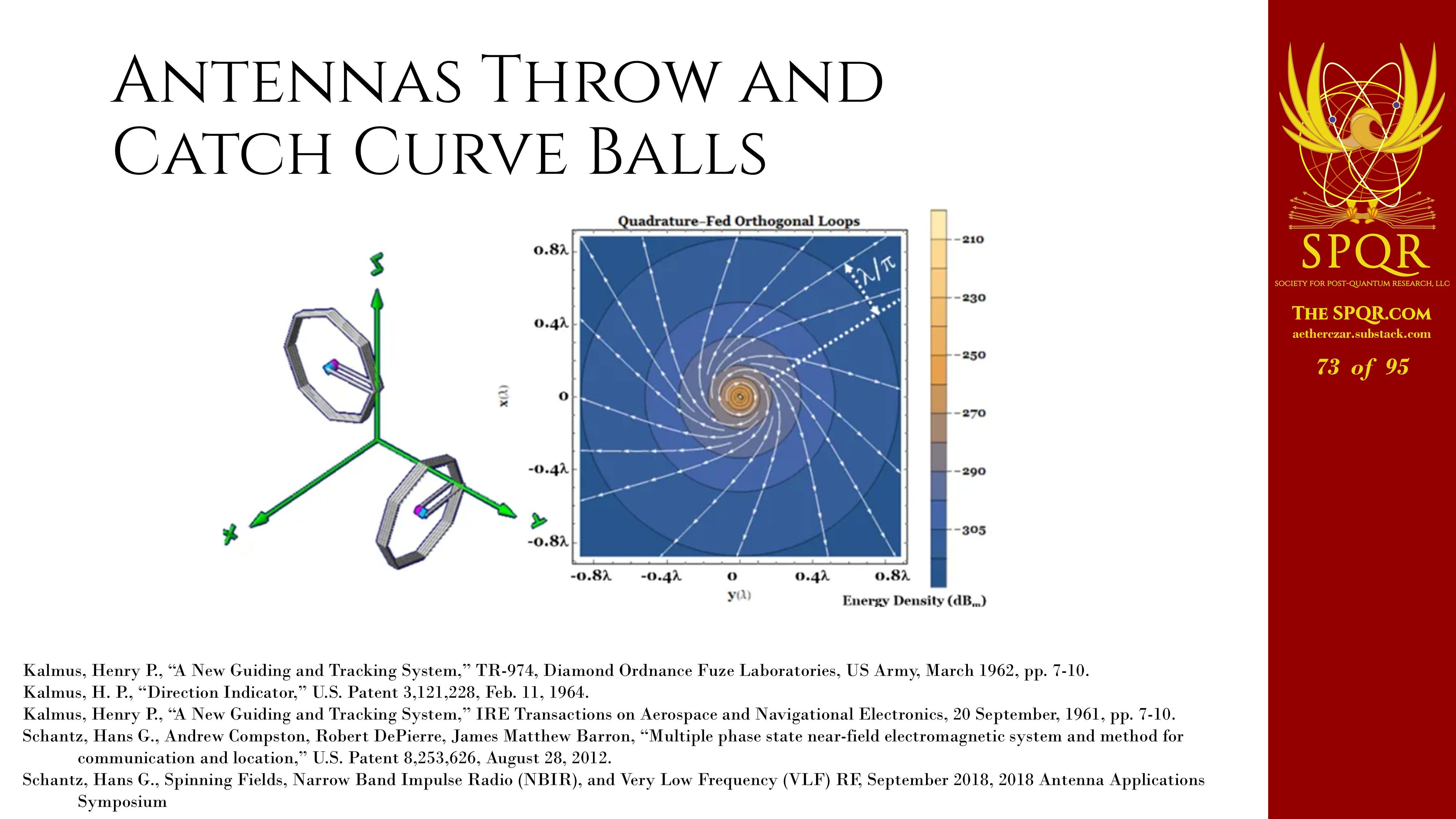
So, if you use direction finding equipment for instance, you’ll discover the bearing you get is offset from the actual source by lambda over pi. I discovered it, only to find that it had previously been discovered back in the 1960s by Henry Kalmas, who was an army engineer, and he also used it to make a location system.

So, this is an example of, you know, if we have science that is repeatable enough and predictable enough to make practical use of it, the term we have for that is engineering. So, this is an engineering example of how energy flow works in a real world system.

A New Paradigm

So, this brings us to a new paradigm of how electricity and magnetism works.

The conventional view is electromagnetism is due to one entity we call a photon. And that photon somehow simultaneously combines the mutually contradictory properties of being a localized particle and a non-localized distributed wave.

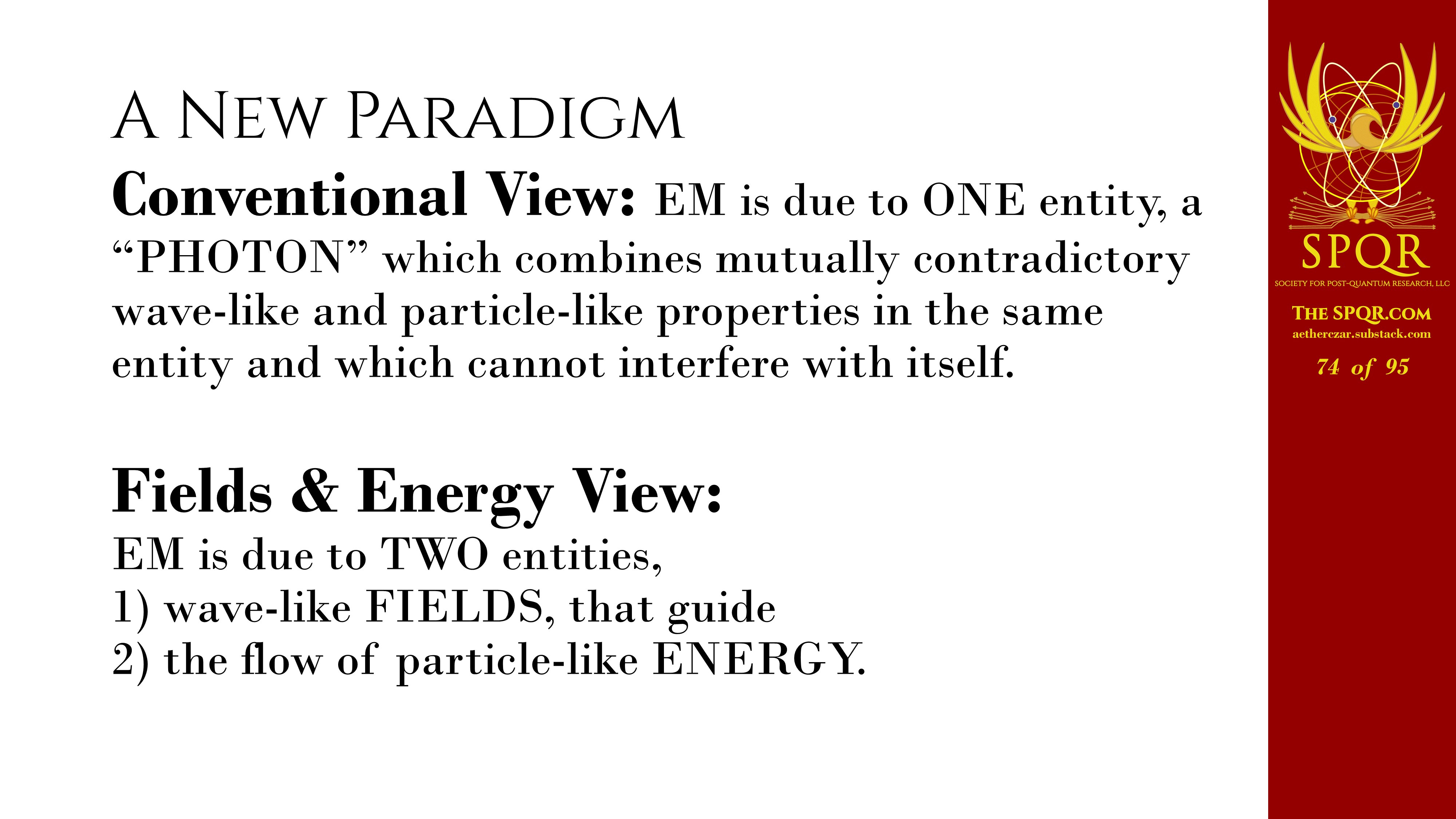
In my view, the “Fields & Energy” view, it’s due to two entities, wave-like fields that guide the flow of particle-like energy. And I’d like to be able to take credit for that, but you can go back to a wonderful paper by Wunscher, Hauptmann and Herrmann in 2002, where they pointed out the basic rules of how fields work versus energy.

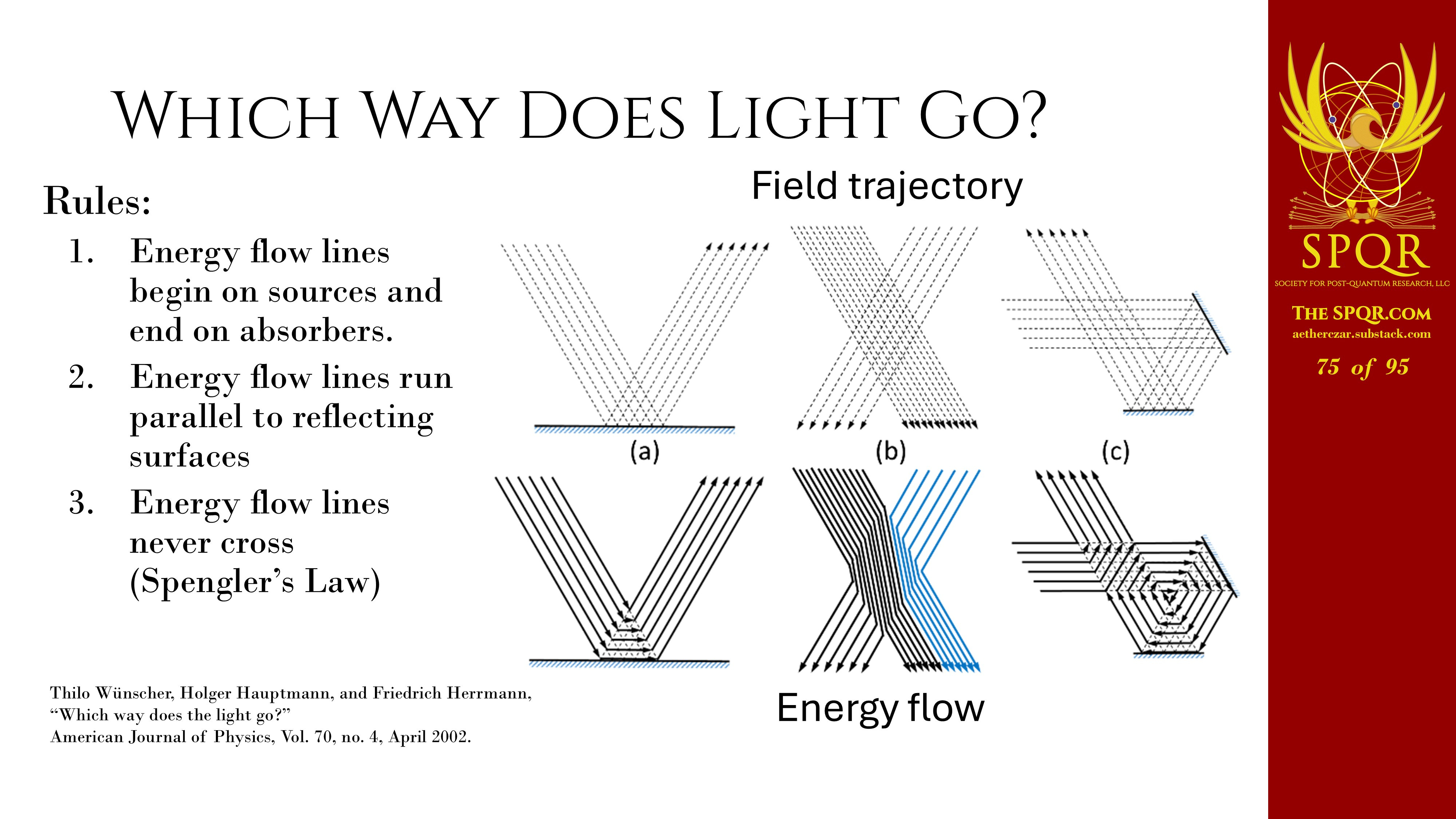
For instance, energy flow lines have to begin on sources and end on absorbers. They have to run parallel to reflecting surfaces if nothing is being absorbed or emitted. And energy flow lines never cross. It’s a vector field. A vector can’t point in two directions at any given point.

In fact, that idea was actually first enunciated back in 1984 by the famed Columbia paraphysicist Egon Spengler who commented, “Don’t cross the streams!”

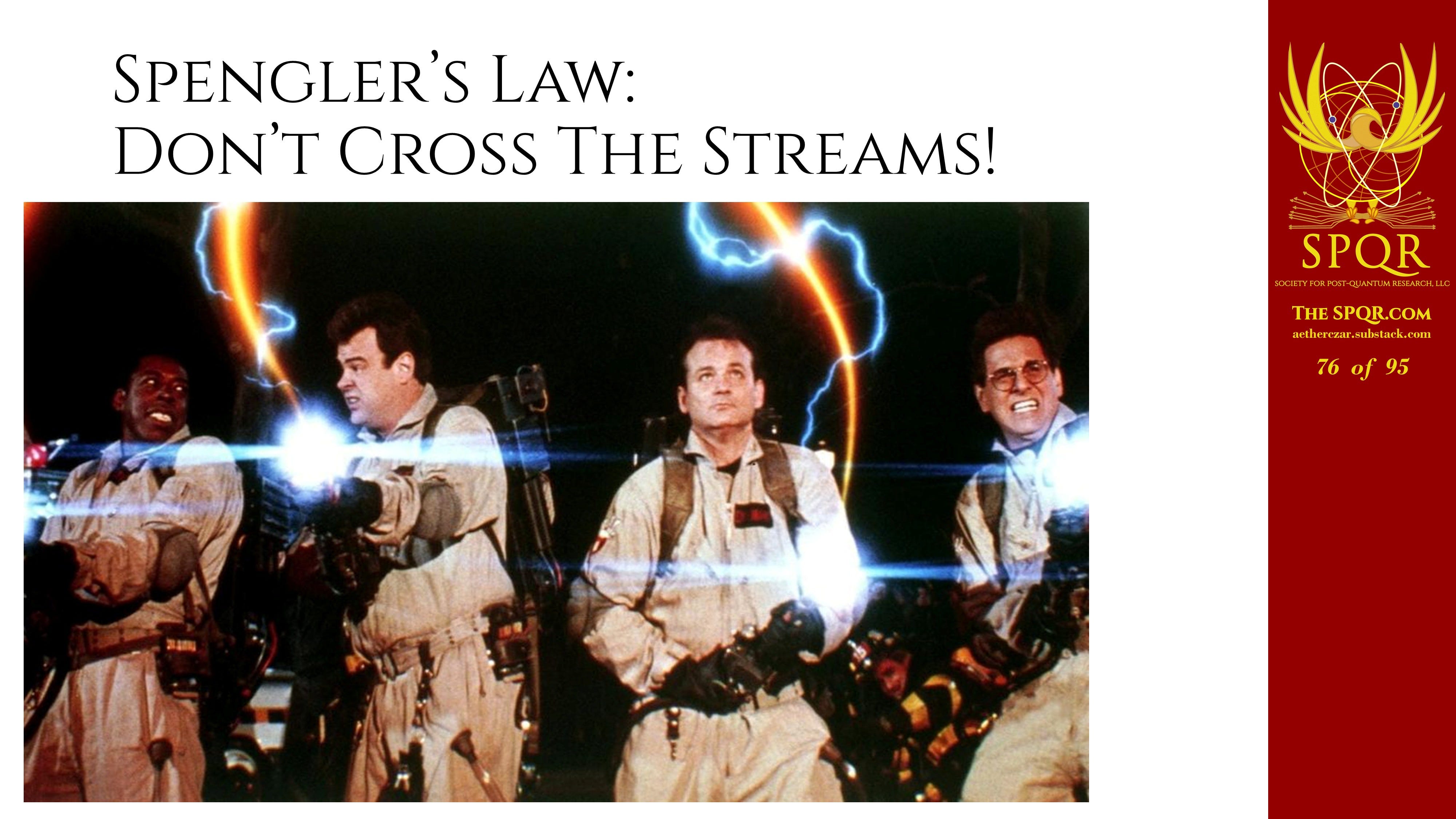
And that relationship, “Spengler’s Law,” I got past the peer reviewers. So that is a peer-reviewed term for this phenomenon.

How Fields & Energy Interact

So, I took NEC [Numerical Electromagnetic Code] and I did some very simple analyses of how this all works, generating a NEC plot of the fields and the energy flow, and then I can give you some comparisons. So, I have this array generating a beam, and you can see all the energy, nice and neat and uniform in the beam.

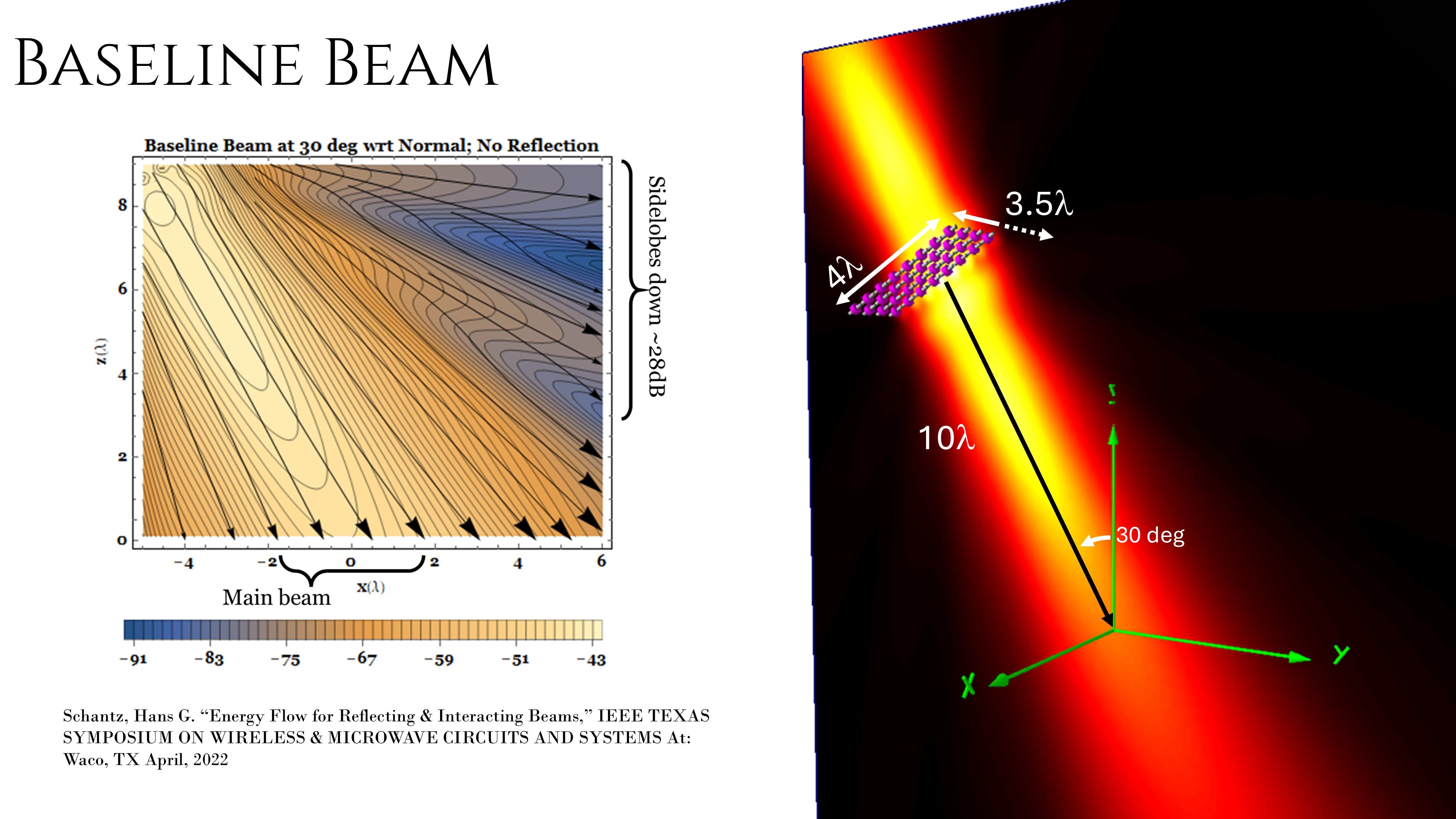
A little bit of side-swiping and exchanging of energy between the side lobes there in the upper corner.

You bounce it off a ground plane and yes, the energy flow is parallel to the ground plane.

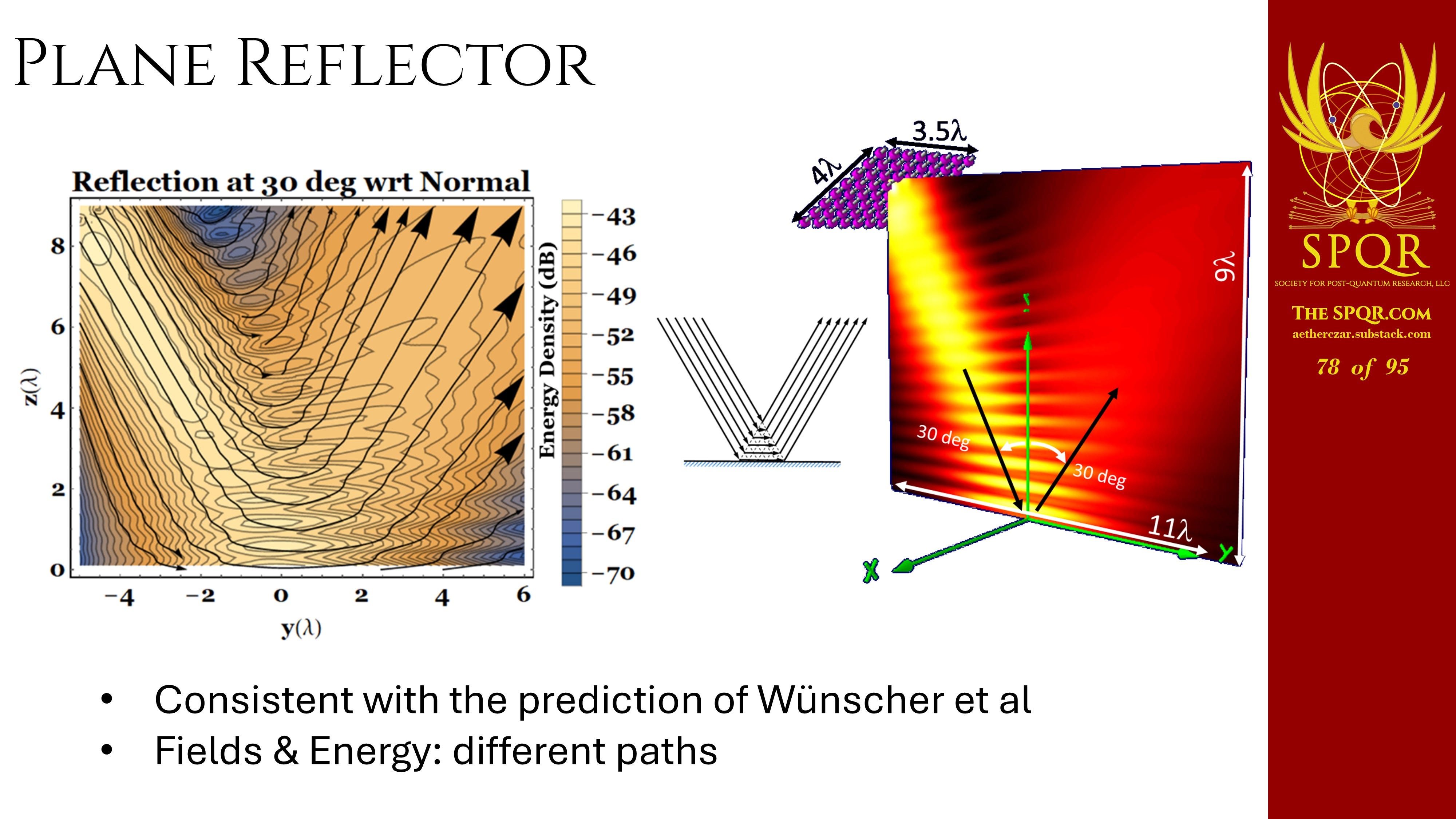
The fields are bouncing off the ground plane, the energy flow is parallel to the ground plane.

You can take a look at that 60-degree reflector example that Wunscher et al. Gave. And you get something similar.

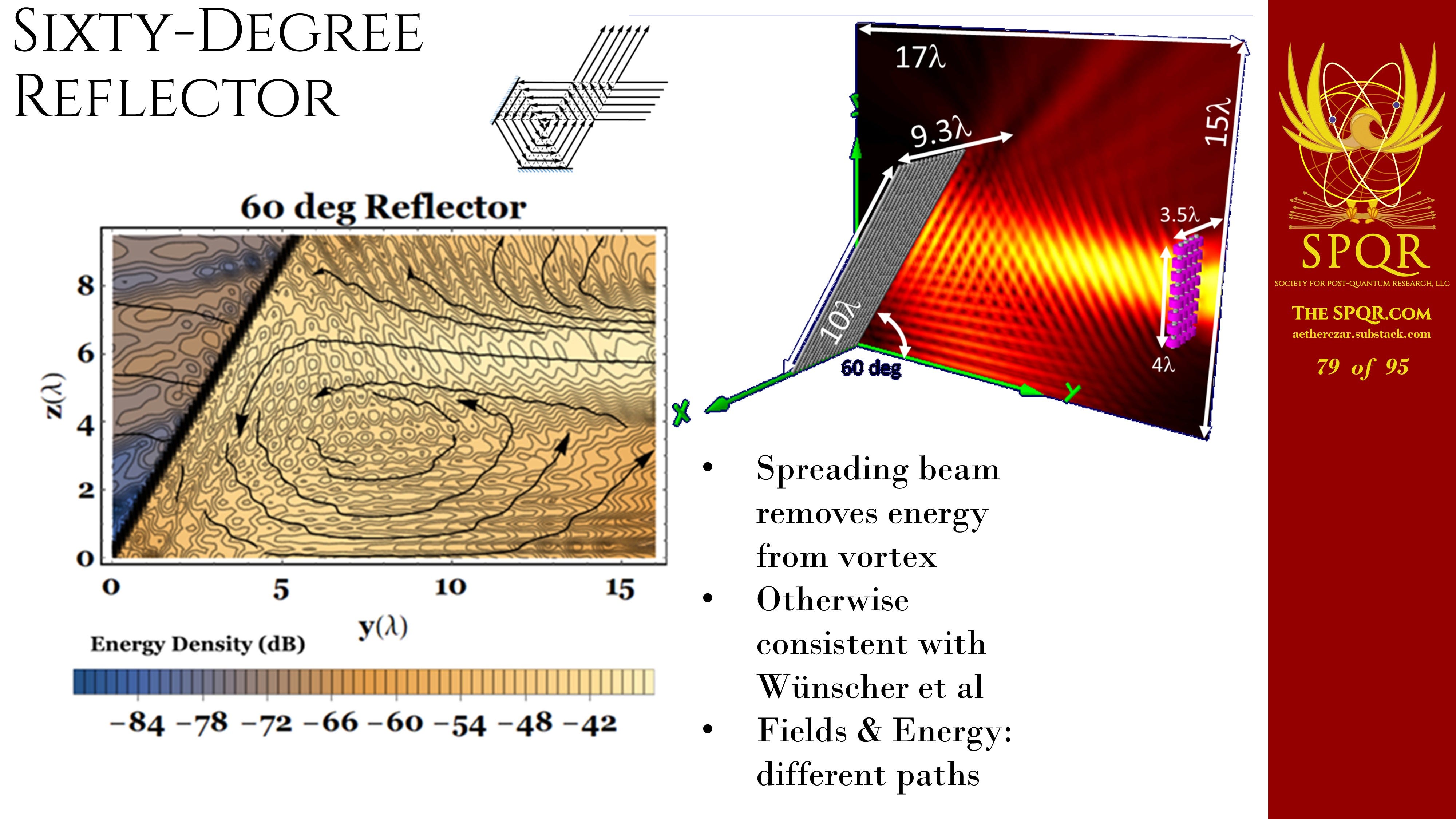
In this case, I have a real-world beam that actually diverges as it progresses. So you don’t get the pure whirlpool in the middle, but you can see something qualitatively similar.

This is an example with an elliptical reflector. Put a source at one focus of a quarter elliptical reflector. And you can see, from a field perspective, you would think the energy flows off, say, in the four o’clock direction.

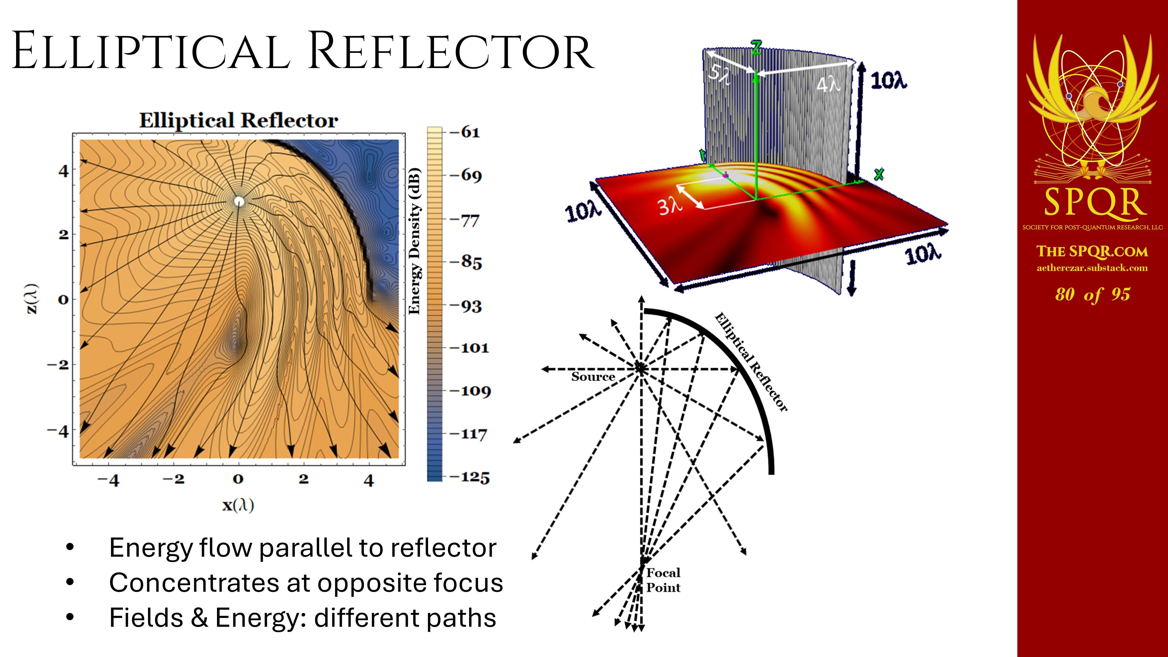
From an energy perspective, you see it’s actually coming off at maybe the two o’clock direction, interacting with the reflected wave from the reflector, and then only ultimately in the far field, ending up in the four o’clock direction.

We can take two beams and see how they interfere with each other with two separate arrays.

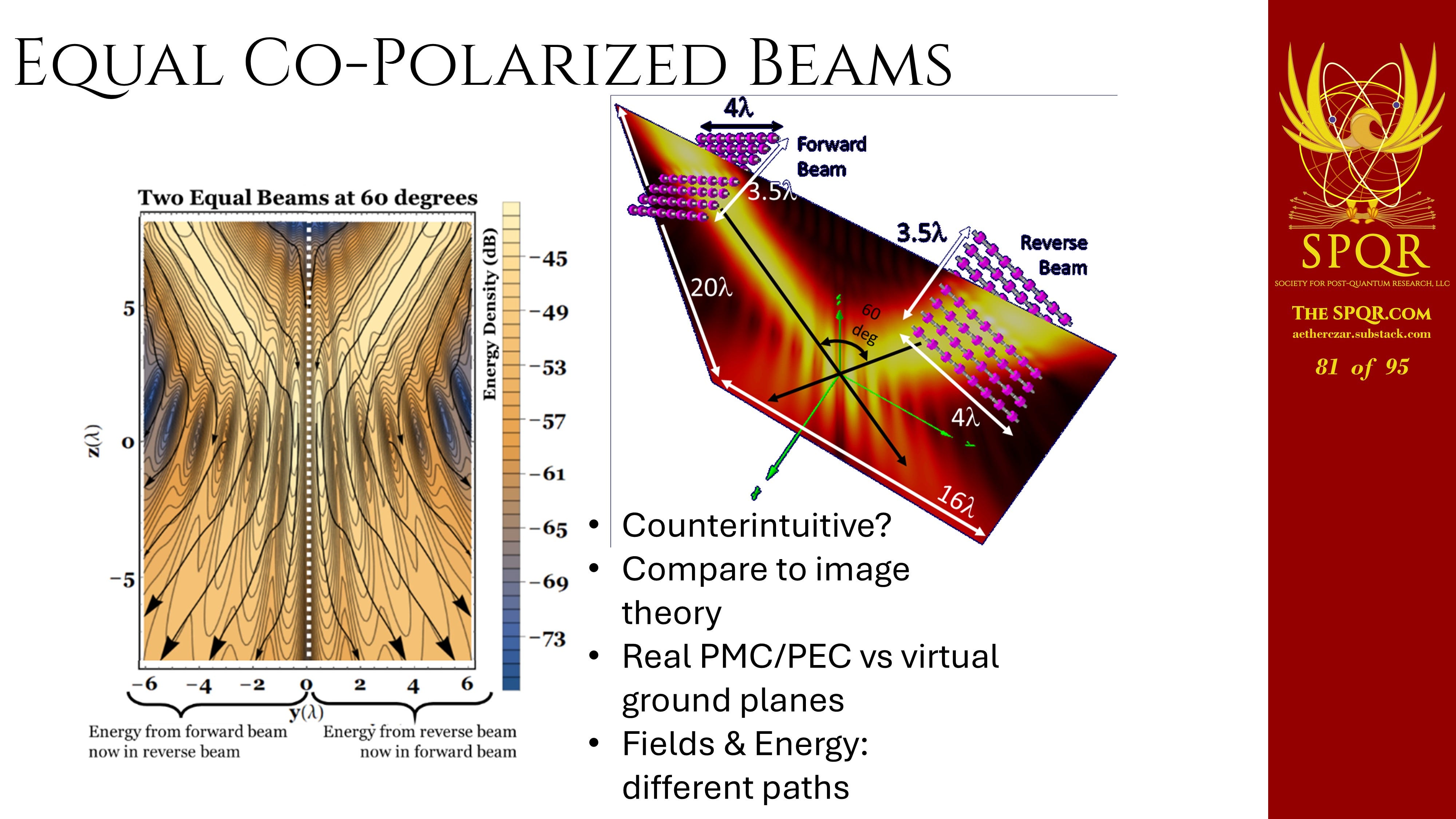
We get that interference pattern since these are co-polarized, but there’s a line between those two equal and opposite beams where no energy flow goes through.

The two beams are exchanging energy.

We can make one beam a little larger and we get that same predicted behavior.

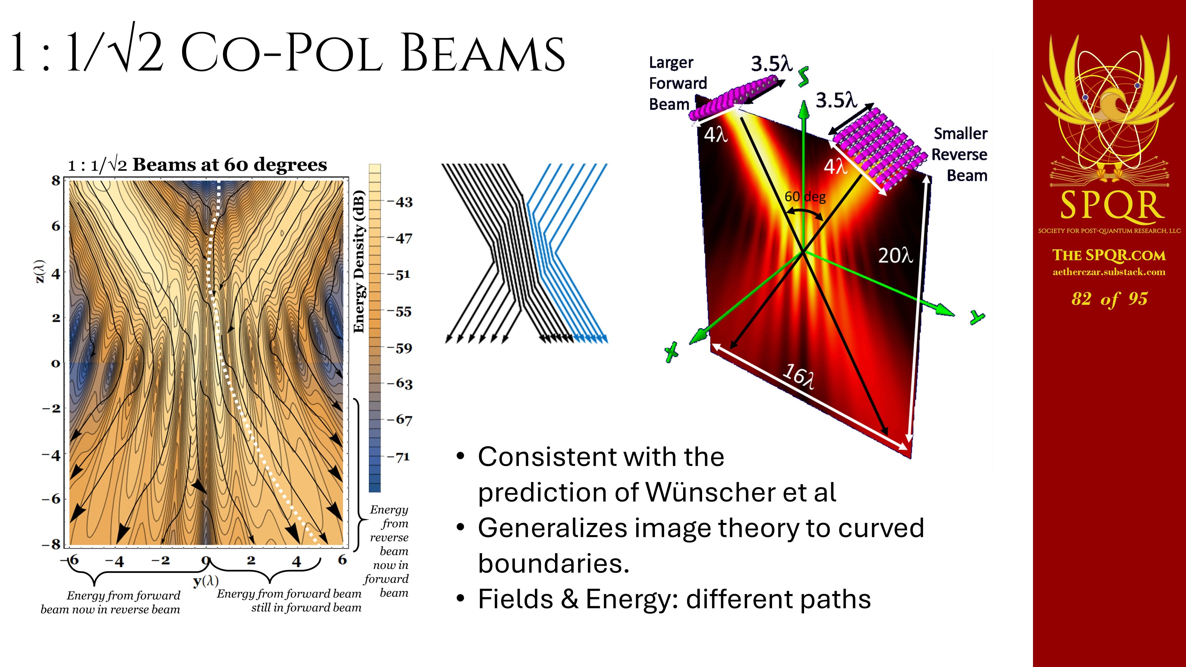
The larger beam sheds enough energy to reconstitute the weaker beam and it absorbs the energy of the weaker beam as they separate and move away.

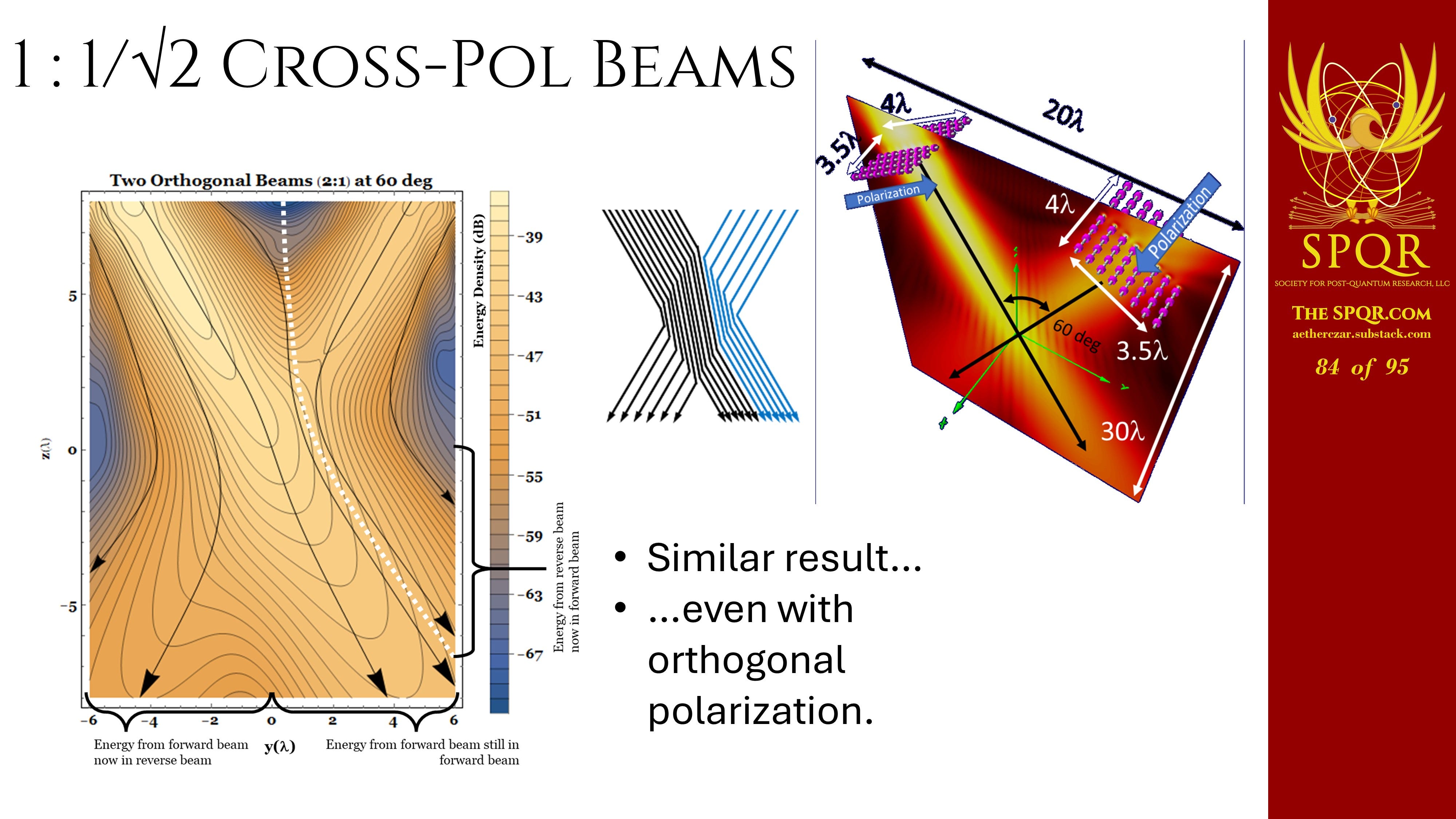
If they’re cross-polarized, there are fewer reflections, and you get an even cleaner and neater picture of this phenomenon, of the two beams exchanging energy…

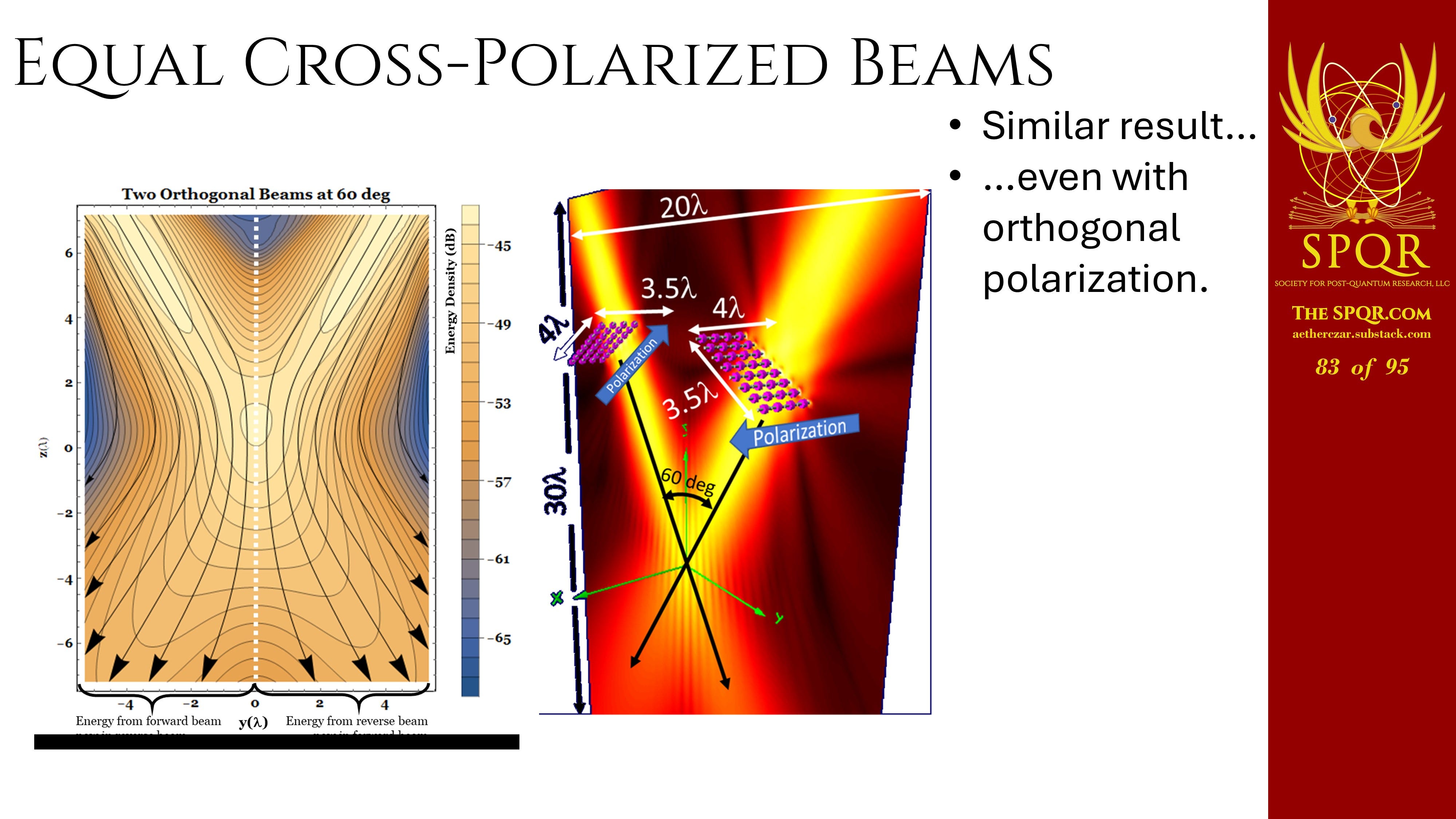
…or a larger beam interacting with a weaker beam.

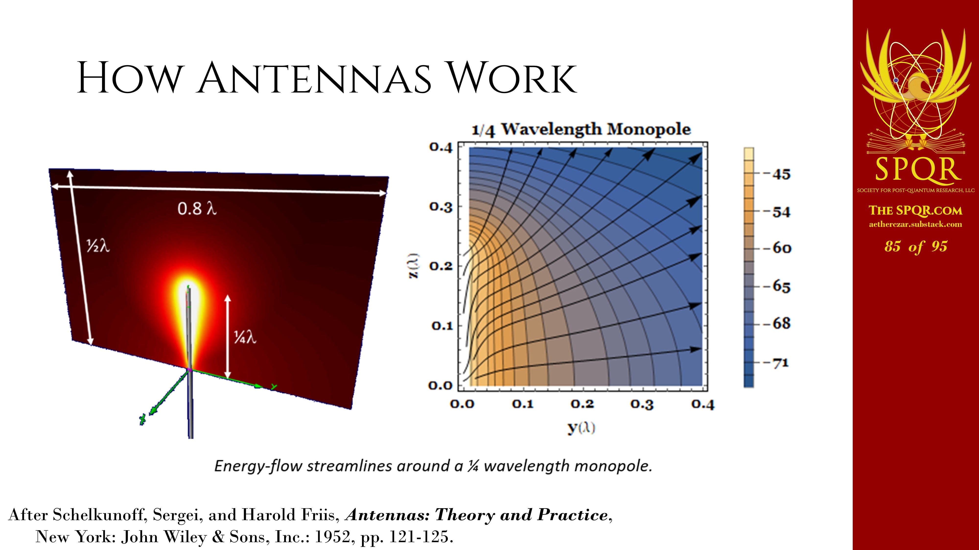
Antenna Applications

This has been used in antenna theory since at least the 1950s, when Schelkunoff and Friis tracked the energy flow along a quarter-wave dipole element to show how it behaved.

There’s an excellent book by Landstorfer and Sacher, Optimization of Wire Antennas where they show how you have energy from a three-quarter wavelength monopole bouncing between a high main lobe and the ground lobe. You’d like to have a low angle of elevation on your radiation.

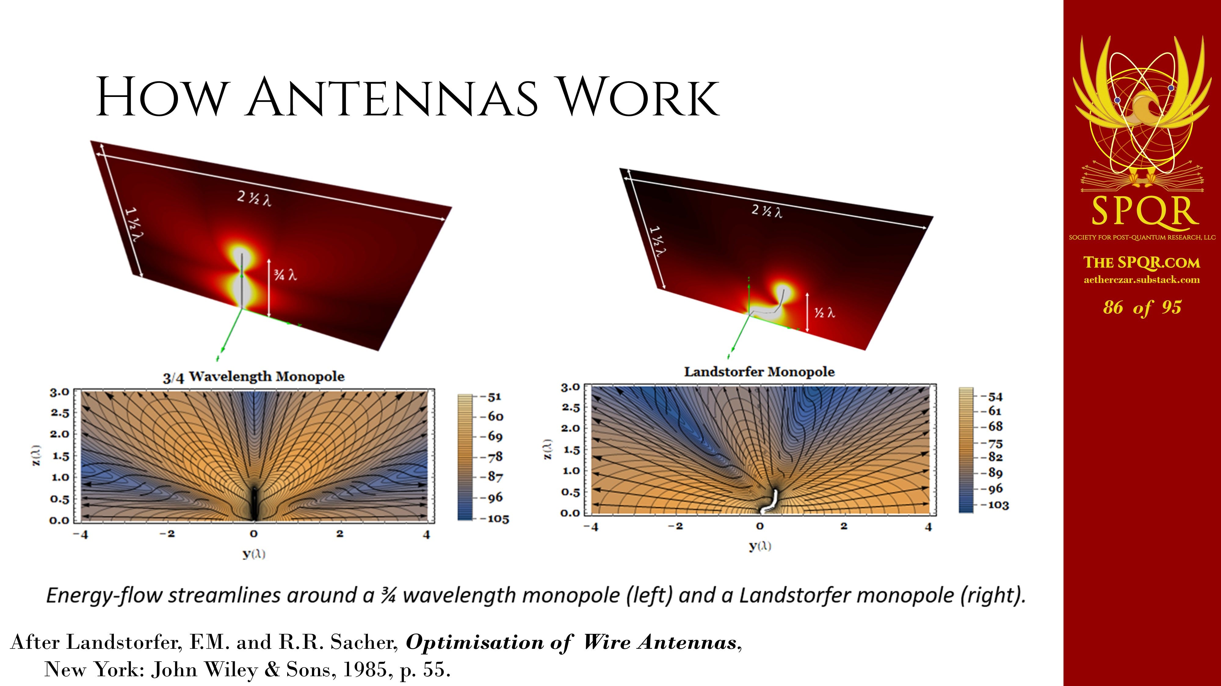
They came up with a way to optimize it in that Landstorfer monopole to get a nice smooth monotonic flow of energy coming out close to the ground.

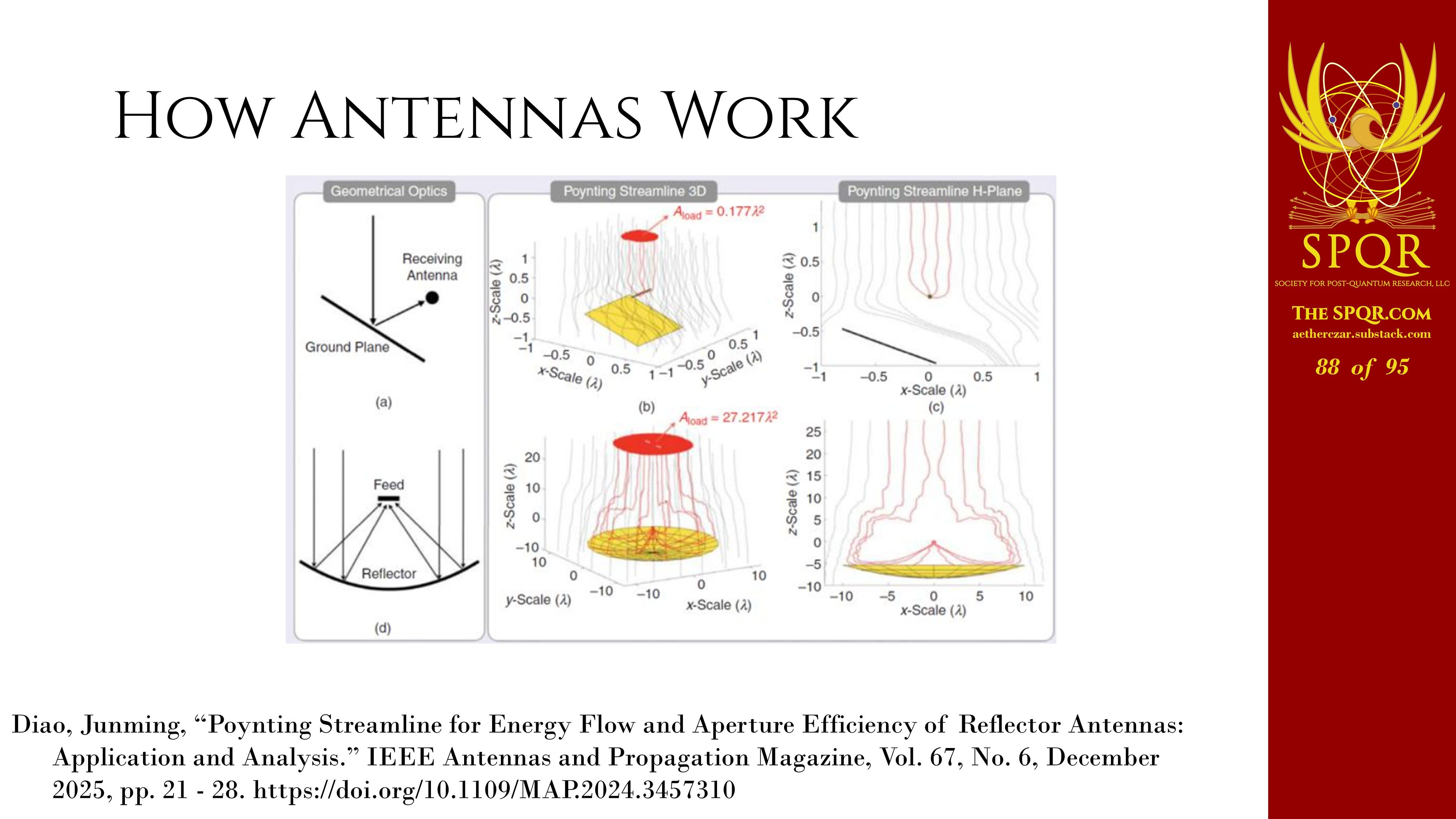
And of course, it also helps you understand how antennas work, how a little tiny antenna can capture a much bigger part of the incoming wave than you would expect from its actual physical size.

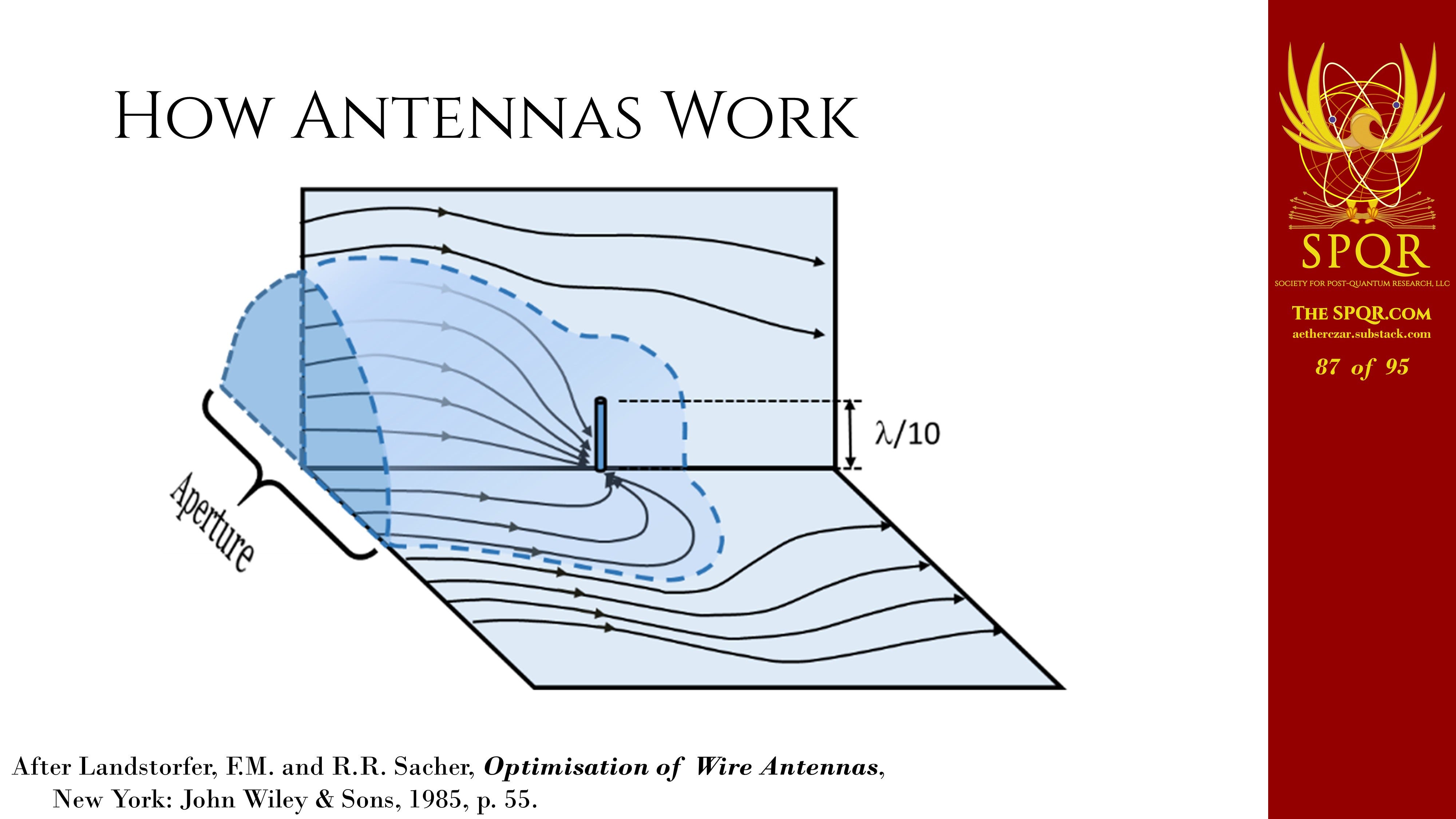
The reflected wave interferes with the incident wave to guide energy into that little antenna.

And this is still being used, for instance, by my colleague Junming Yao at Mississippi State University, where he’s using that to show how reflector antennas pick up energy and what the effective aperture is and how the energy flows around parabolic and planar reflectors work.

Connecting Antenna Physics & Quantum Physics

An excellent example of this disconnect between physics and engineering is just in the last year I realized I don’t think anyone has ever taken a look at the hydrogen atom to see if it corresponds to the rules we all know for electrically small antennas.

And it turns out they do.

And apparently physicists are unfamiliar with how electrically small antenna limits like Chew Harrington work.

And engineers aren’t necessarily familiar with decay times and Einstein coefficients.

You put the two together, and you can show that atomic processes obey the Chu-Harrington limit.

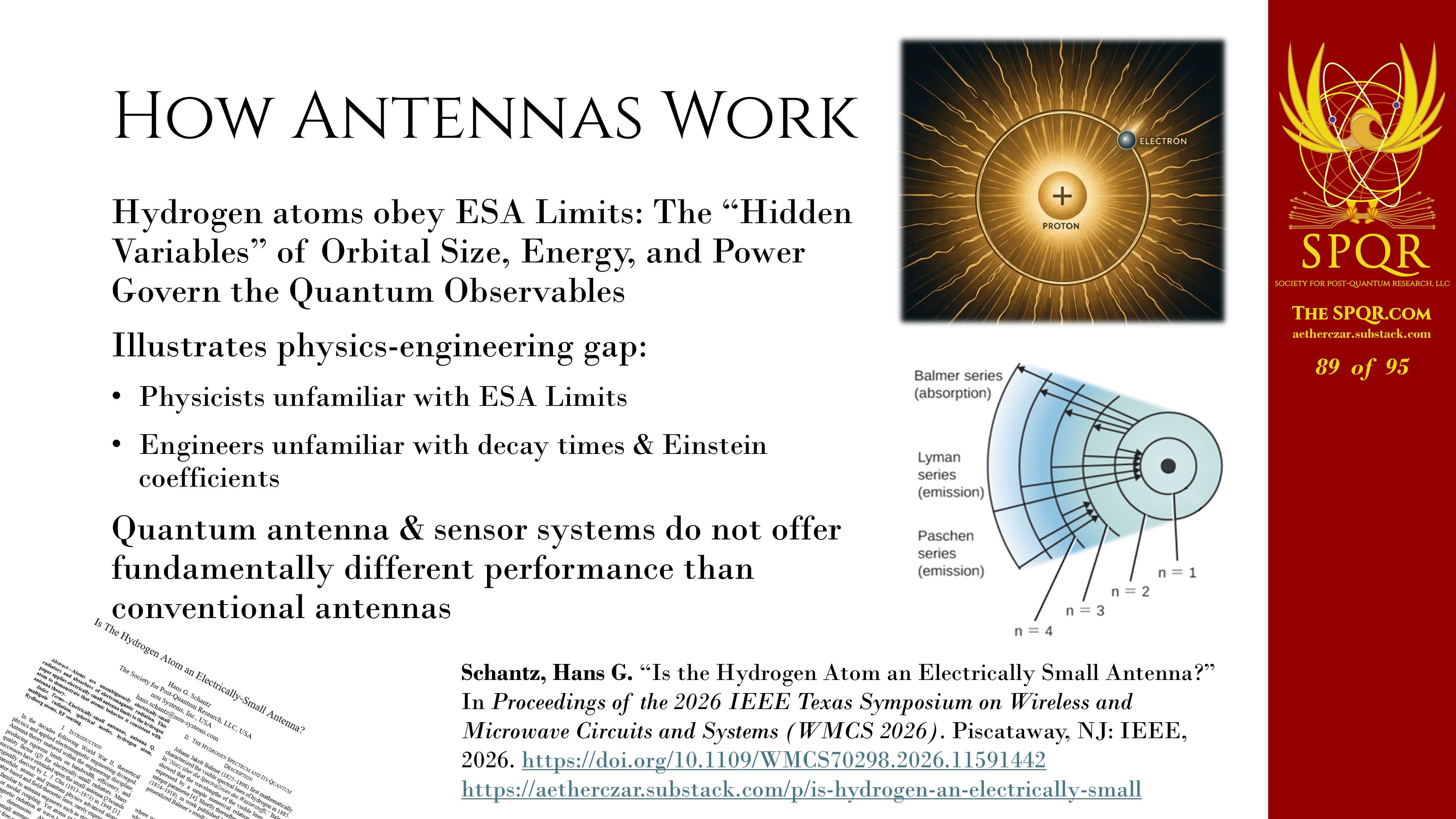
So, there’s a lot of talk about quantum antennas and sensors having miraculously better performance than conventional systems, but they obey the same conventional rules.

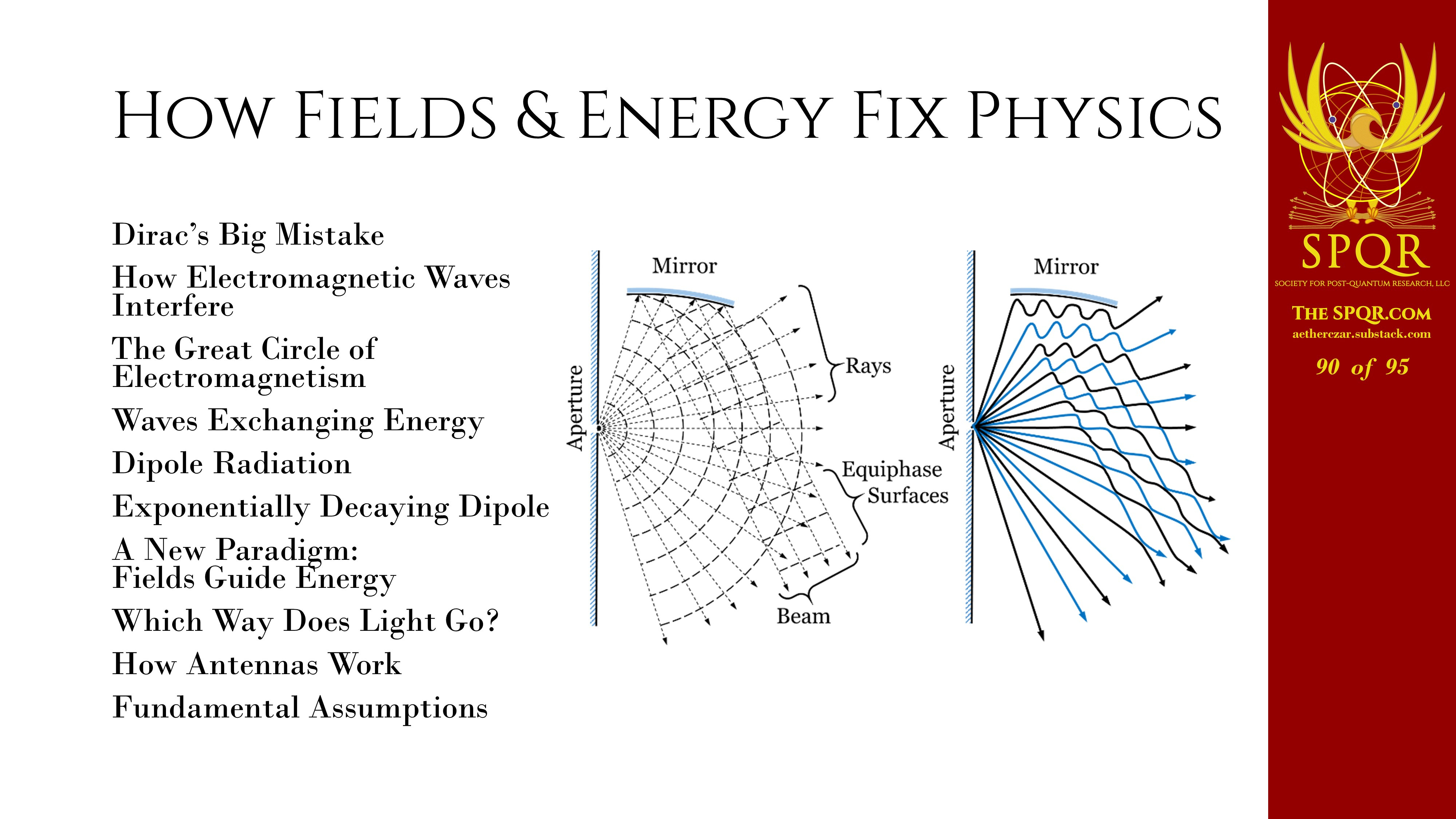
So, I’ve talked about how Fields & Energy fix physics in my view, how you have these two pictures of waves propagating through, you can treat them optically like rays, and how they give rise to a different picture where you can track the flow of energy through your system and give you another perspective on things.

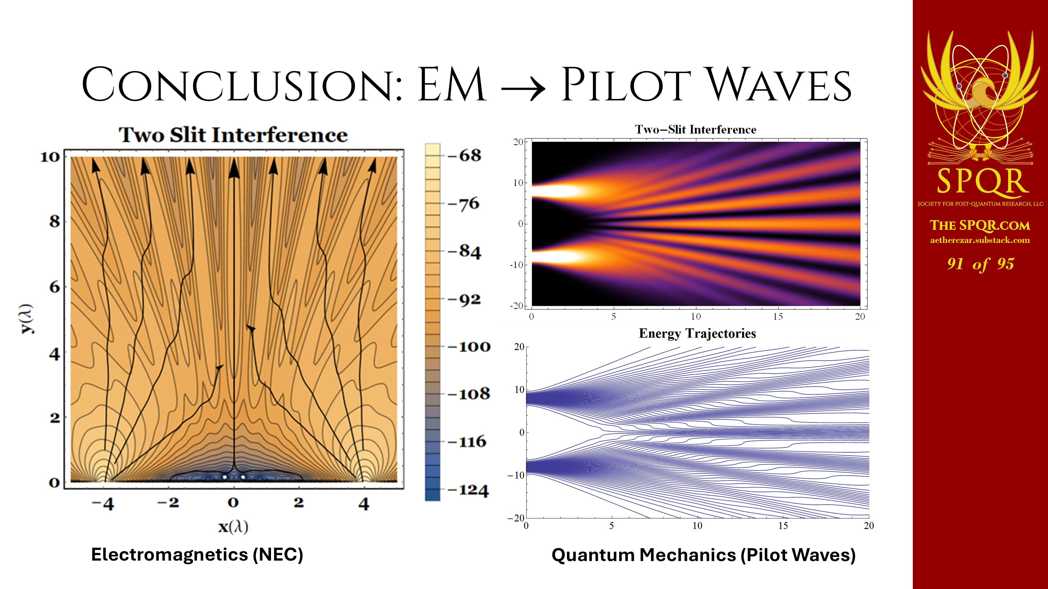
So, when I take a look at an energy flow perspective of how energy works in an electromagnetic system from two tiny apertures, and I compare that to the quantum mechanical predictions of the pilot wave trajectories from pilot wave quantum mechanics, I take a look at those two pictures, and in the words of the internet meme, I think they’re the same picture.

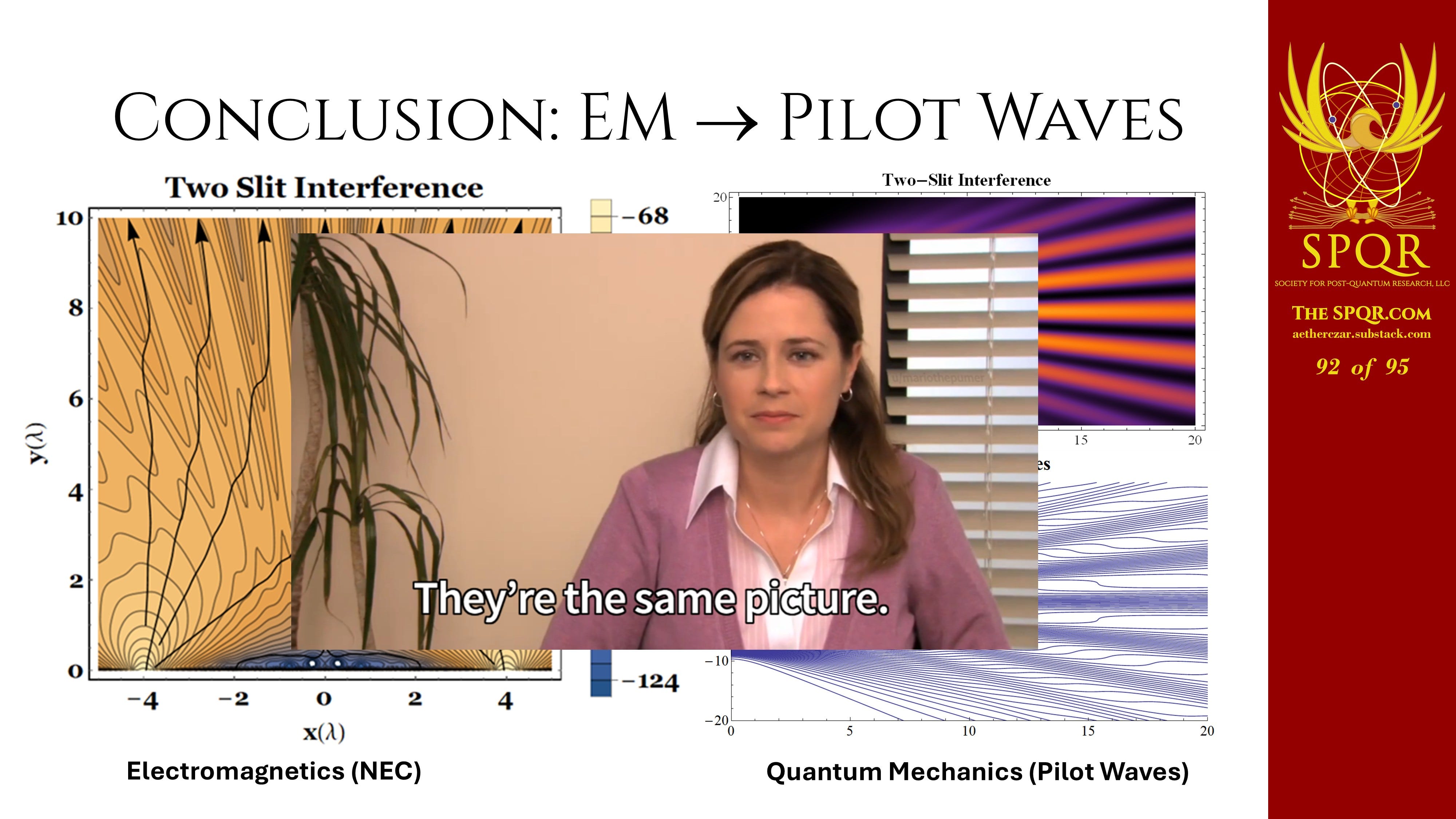
I think that the pilot wave approach is the logical consequence of applying electromagnetic energy flow relationships to how light and how photons and energy move in our electromagnetic systems.

John Wheeler, writing a few years before I knew him in his book, Journey into Gravity and Space-Time, said, “Someday surely we will see the principal underlying existence as so simple, so beautiful, and so obvious that we will all say to each other, how could we have been so blind so long?”

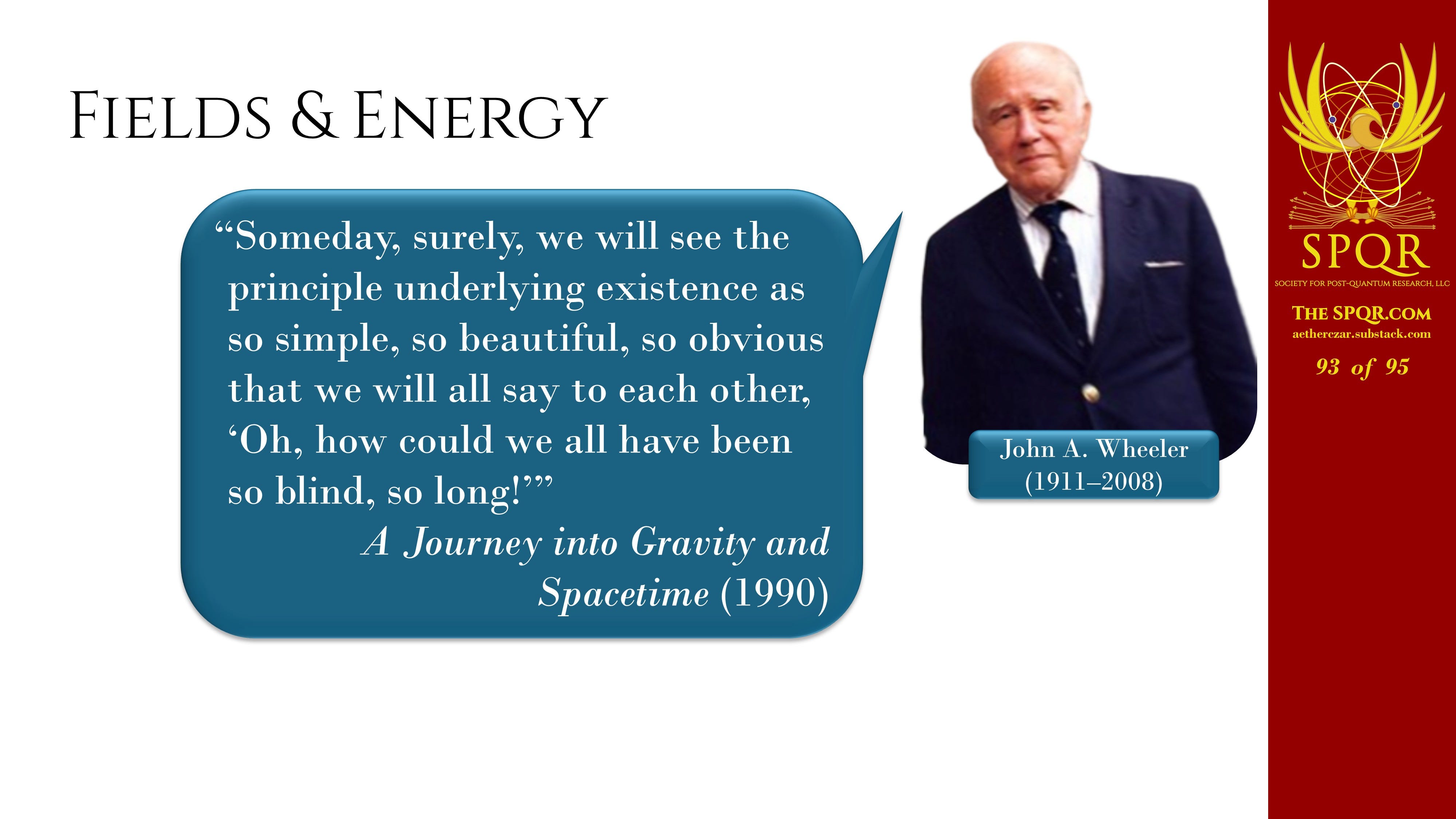
I hope this “Fields & Energy” perspective helps bring us closer to that day.

So in summary, I’ve talked about fundamentals and origins of electromagnetism and walked through where physics went wrong and how electromagnetism and quantum mechanics work.

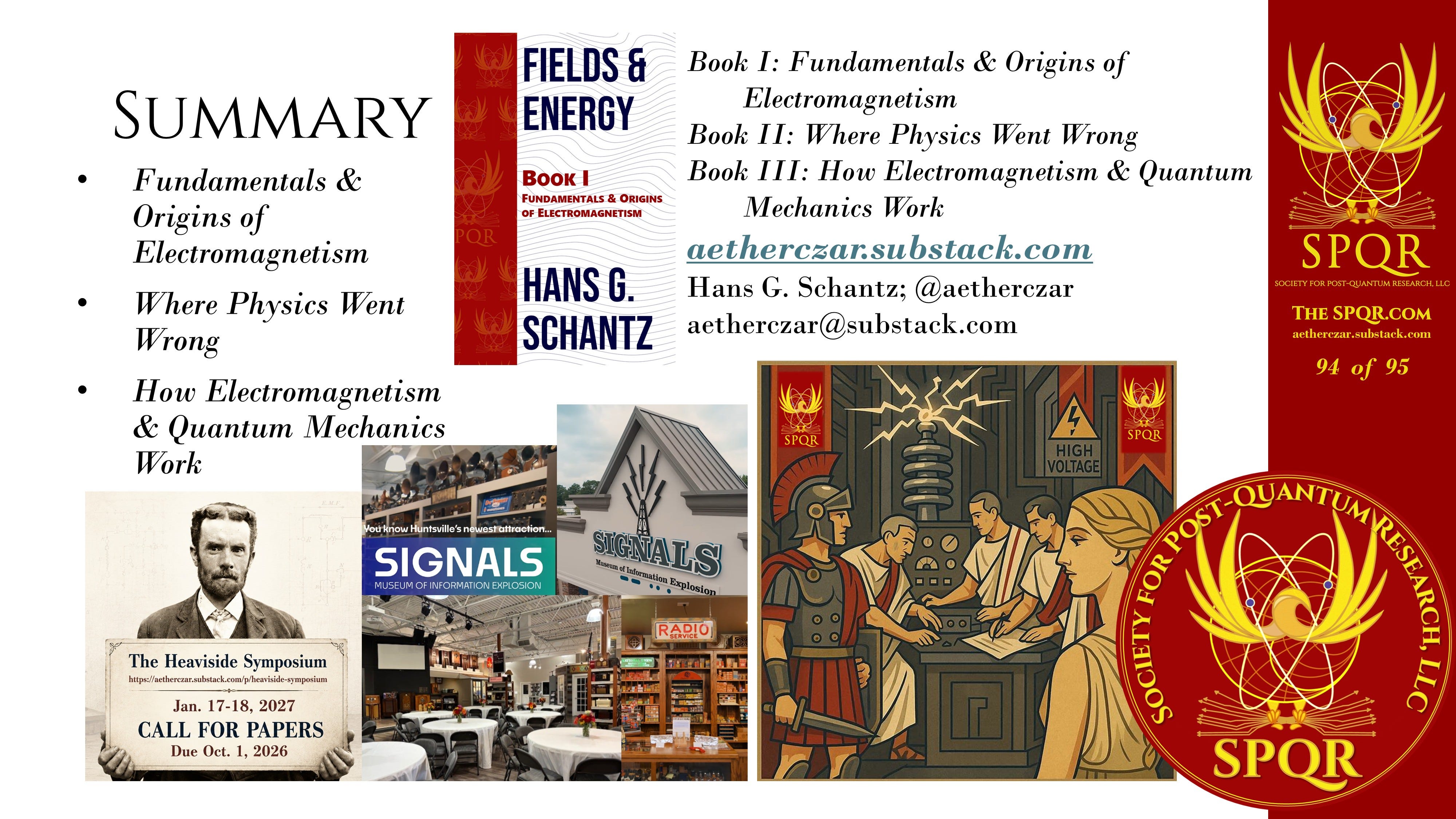
If you’re interested in this, I can recommend my book, Fields & Energy.

The contents of Book 1 and most of the contents of Book 2, which has not yet been released, are available on my Substack at aetherczar.substack.com.

I have a bunch of references there…

…and I’ll put up the slides when I get a chance to get back home and organize them. Hopefully the video of this talk also [And here they are, two weeks later!].

And if you’re interested in exploring these ideas further, we’re holding the Heaviside Symposium at the Signals Museum in Huntsville, Alabama, MLK Day weekend.

I hope I’ll be seeing some of you there.

And I’ll be happy to take any questions that you have.

Questions & Answers

Benoit: Let’s thank the speaker first for a brilliant keynote. Thank you, Hans. So, great timing. We have time for questions. Who wants to raise a question to Hans? Okay, Chuck, coming with the mic for you.

Chuck: Great conversation. Thanks so much for your talk today. When I was in grad school, I studied under Dr. Bessiere, who was one of my professors at Virginia Tech, and I had to do a paper on the Aharonov-Bohm effect, where it was trying to provide a physical kind of effect?

Hans: Yes, it is the same Bohm. The question is about the Aharonov-Bohm Effect.

That Bohm is the same Bohm who did the revitalization of the pilot wave theory. The basic idea is they have two slits and they run electrons through the slit, but they put a solenoid in between the two. That is confining magnetic fields. And what they discover is in the mathematical representation of… I guess it’s the Schrodinger equation they use for that… there is a term where you’re looking at the magnetic vector potential A and how it interacts and causes phase shifts in the electron trajectories. And that is an observed phenomenon.

And my question about that was always, well, wait a moment. Yeah, solenoids confines magnetic flux, but there’s an equal and opposite amount of flux coming out that’s distributed somewhere. And I wasn’t really happy with the experiments that I saw on that.

Turns out in the 1980s there was a marvelous experiment done by a Japanese researcher, I’m very sorry I don’t remember his name, where he took a small toroidal magnet and plated it in a superconducting material. To a high degree of confidence, closing all the magnetic fields in there and discovered that, yes, the electron beam going through the center of that toroid did show an offset.

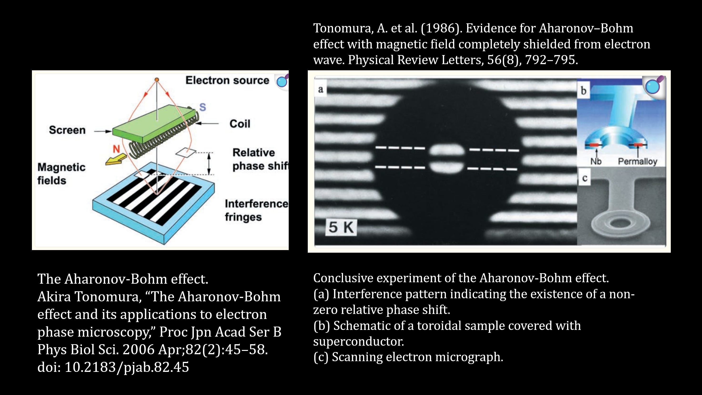
Note: Tonomura, A. et al. (1986). Evidence for Aharonov–Bohm effect with magnetic field completely shielded from electron wave. Physical Review Letters, 56(8), 792–795.

So it does seem to be a real thing. It is very intriguing. It suggests that the potential is not just a tool, a mathematical tool for calculating fields, that it has some physical, real-world influence.

So excellent question. Thank you.

Benoit: More questions. And we need to challenge Hans to see if we can find one question he cannot answer.

Question: First of all, thanks for the great question. And I have a question. You see one slide talking about the two waveforms. Something that’s crossed over. Some kind of bounce back. Why is that?

Hans: The two waveforms that are...

Question: ...interference with each other. [Indistinct].

Hans: Yeah, what’s happening is basically the fields pass through each other at the speed of light.

But if you take a look at how they interfere with each other, you’re getting places where you have electrostatic or magnetostatic energy. The energy velocity is actually slowing down. And when you look at the big picture of that system of how that works, you have energy being exchanged between the two beams. So, fundamentally, we like to think of, well, for instance, if you, as engineers, if we want to understand a cell phone and how that cell phone works, what we’ll do is we’ll say, okay, I’ve got a direct ray to the cell phone tower. Maybe I’ve got a multipath bounce. Those are the two principal components.

Say I’m in an open field and I add them up. I get the sum and the phase difference and that predicts the link and I can predict exactly how much power I have at the other side of the link. And that’s good for an engineering calculation.

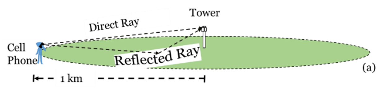
But if you step back and ask yourself what’s really going on in reality, you have to keep in mind there is a kilowatt per square meter of electromagnetic energy coming down from the sun. And in thermal equilibrium, an equal and opposite amount of electromagnetic energy of infrared electromagnetism coming up from the ground.

And what happens is that little tiny tickle of a cell phone signal is going through those vastly greater flows. Whatever energy is in it is very quickly going to get swept away. That little tickle of a cell phone signal radiates through there and somewhere near the receive antenna it captures and bumps a little bit of whatever energy it happens to find into the receive antenna.

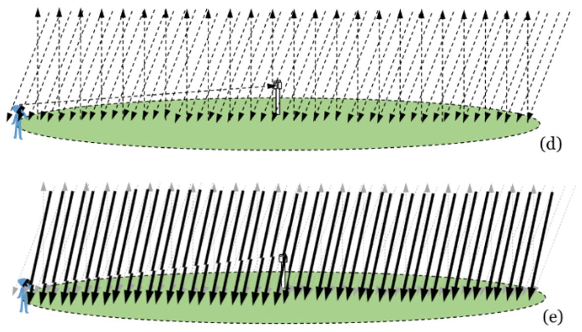
So it’s a completely, the “Fields & Energy” approach is a completely different way of looking at a system. Now there, hey, it’s much easier. Just take the two rays, add them up, and do the calculation.

But if you want to ask yourself physically what’s really happening in the real world system, you’d have a picture more like that, you know, those energy forms.

Question: Showing the energy.

Hans: Showing what?

Question: The energy, energy, energy. Energy, not the EM here.

Hans: Yeah, this is the plot. Well, the plot on the left is showing the, I think, the electric field intensity, and the plot on the right is showing the energy density.

Question: Ah, okay. So, one more curve, can you go to the other one? It can have a challenge somewhere for... How they...

Hans: This is when they’re co-polarized, so we get a lot of interferences and nodes.

Question: Some just crossing each other, not a reflection wave.

Hans: Oh, the question is, why can’t we just have two flows crossing each other?

Question: I see some picture has crossed each other. In the early slide, probably.

Hans: There are some that may look like they’re crossing, but when you do a detailed analysis, they’re not.

Benoit: I think maybe the question is between this picture and the other one, and the difference is here you have an unbalanced distribution of the energy, right? There is one smaller beam.

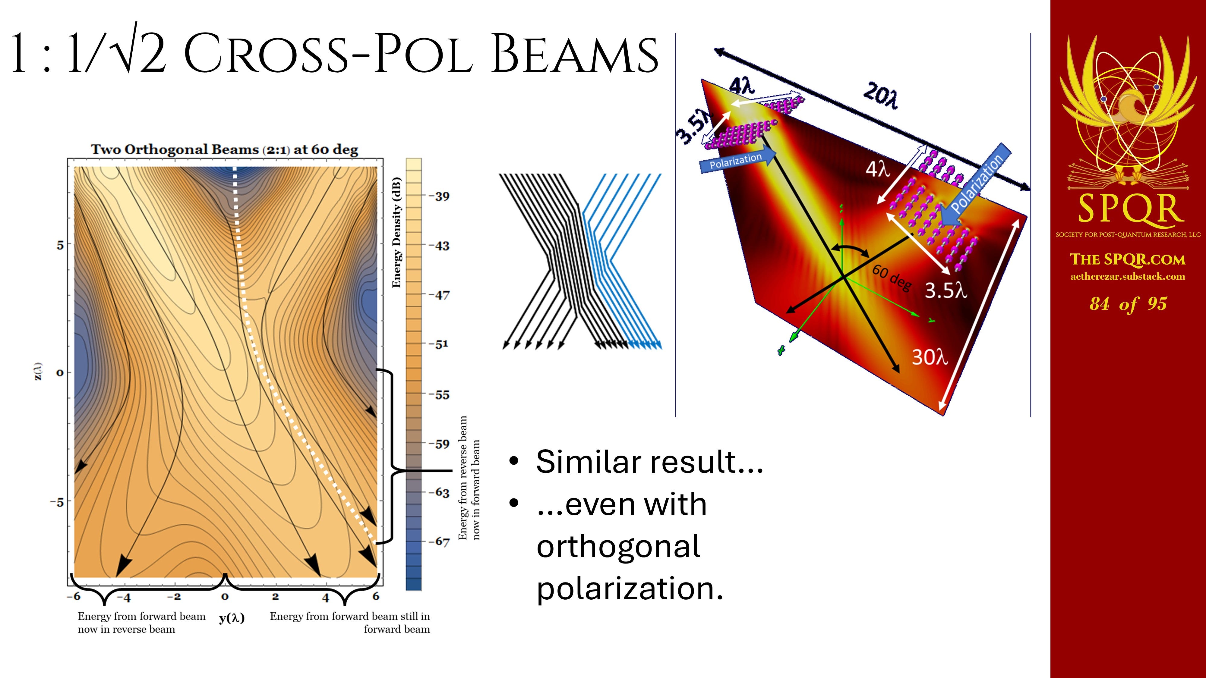
Hans: Right, one beam is weaker than the other here.

Benoit: One beam is weaker than the other, and somehow then there is a kind of crossing of energy because there is one beam that has sort of a dominant Take on the energy, right?

Hans: Right. The stronger beam is basically capturing all the energy from the weaker beam here.

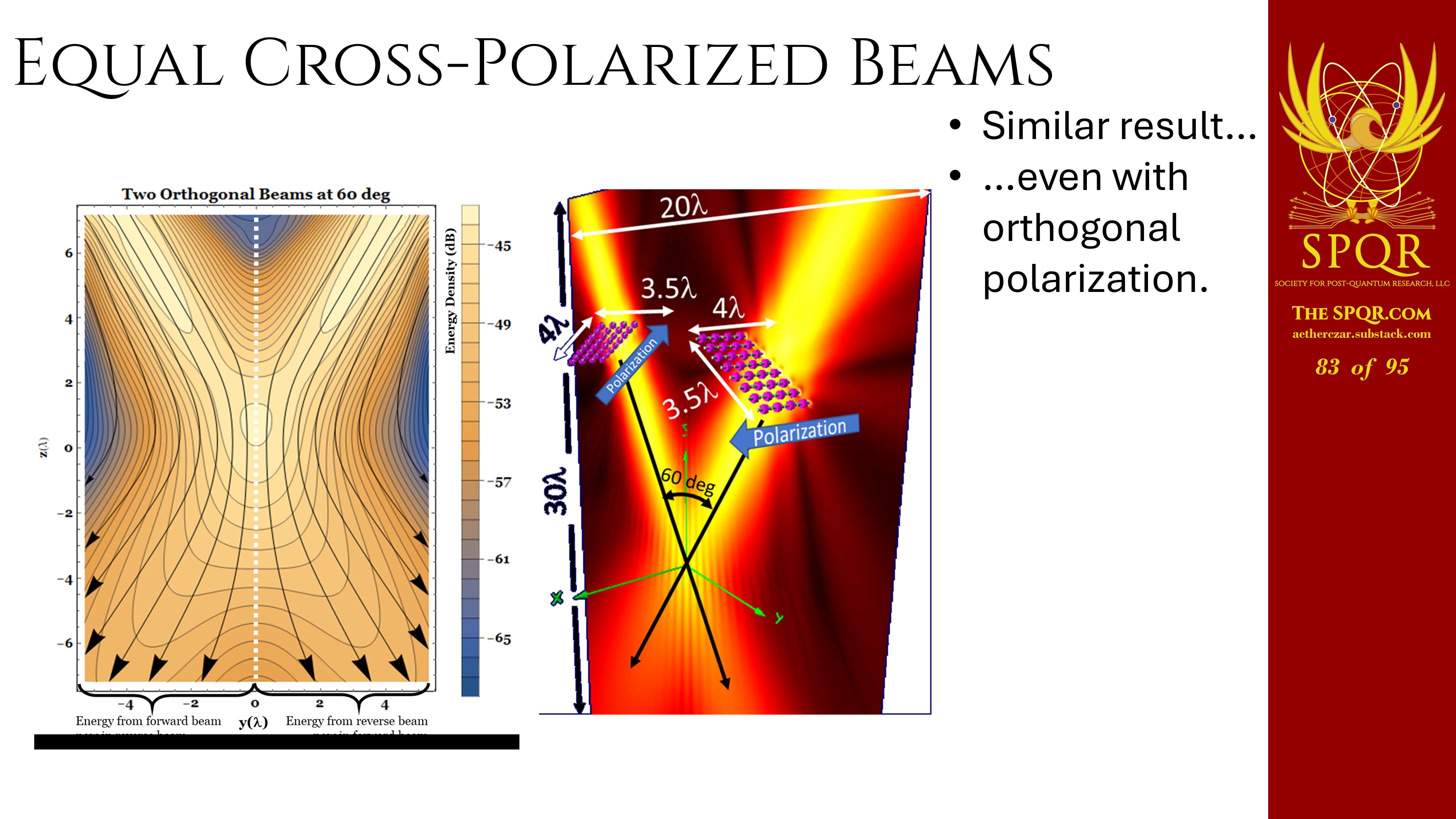
Benoit: Exactly. And when they are identical, then you have sort of, and they look like bouncing back, right? Yes. Because there is this causality or causal surface, I don’t know how you call it exactly.

Hans: And in fact, a good way of thinking about this is image theory. In image theory, we want to understand how a source interacts with a ground plane.

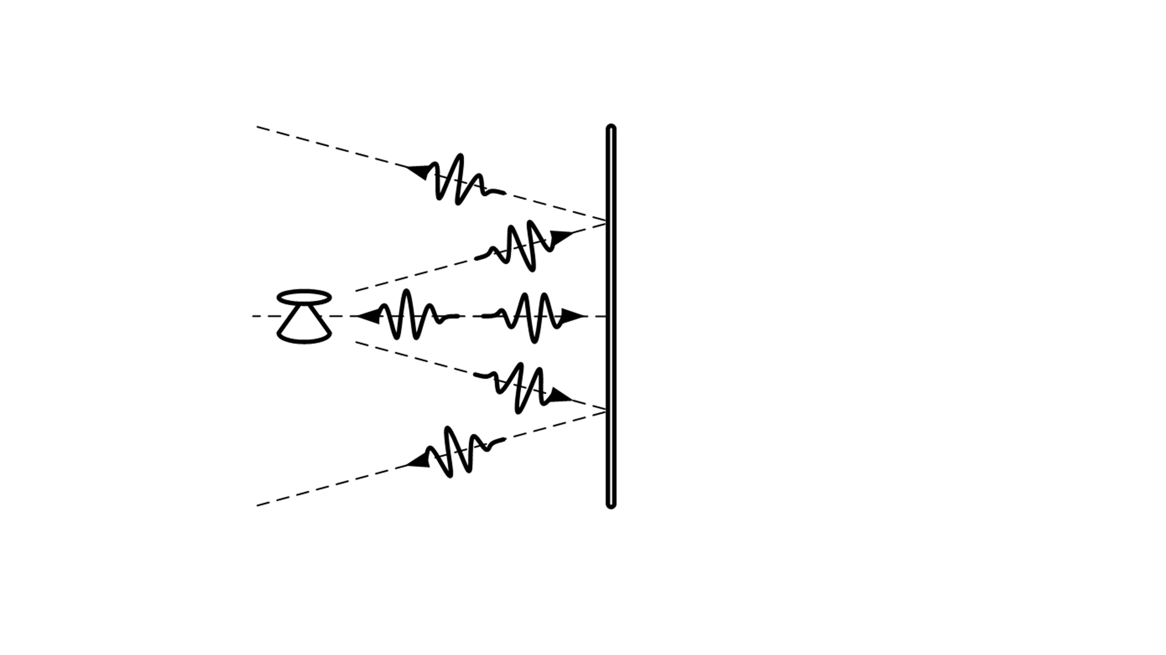
So we put a virtual equal and opposite source on the other side, we add them up, we get the solution, and that gives us the boundary condition for the ground plane where the fields are bouncing off it and there’s no energy there.

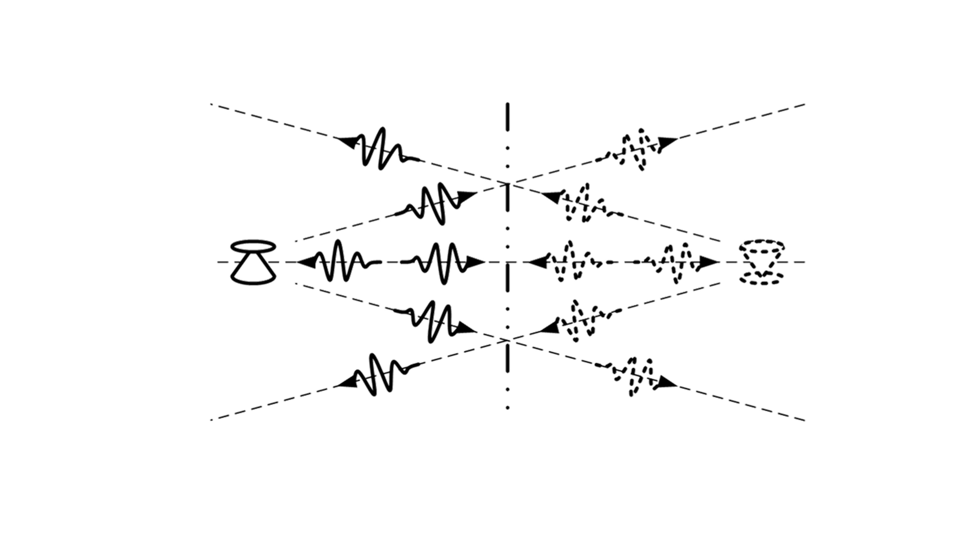
Well, let’s remove the ground plane and put an actual equal and opposite source. We have the exact same math, the exact same calculation, the exact same no energy is going through the plane.

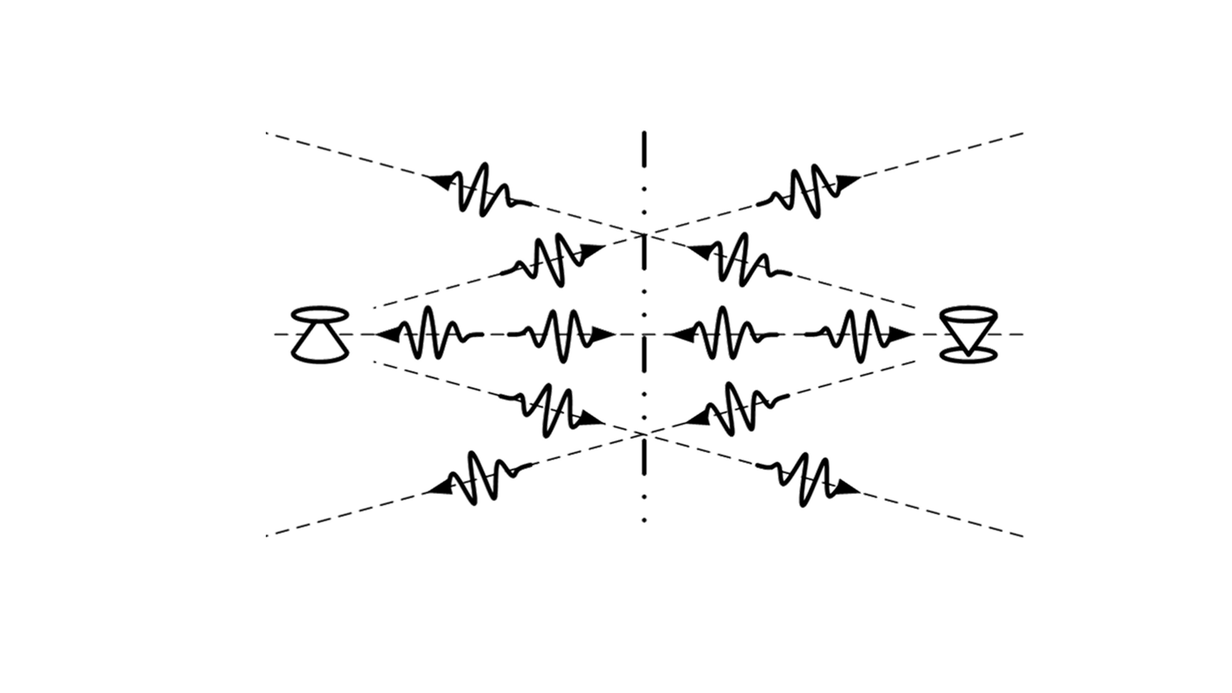
I argue it has the same interpretation that the energy is bouncing off the virtual ground plane that’s set up by that equal and opposite source.

Benoit: Any more questions? We have time for a couple more.

I start here in the middle.

Question: So, I work currently on an open source full-weight software. But before this, I worked at Thomas, where I made ray-rich demo systems. And I was trained by someone who worked there for 40 years. And he taught me that a good engineer needs to be able to switch between thinking in fields and thinking in transmissionary models.

But I would love to also ask. So I’m wondering, is there anything more magic to this than just essentially looking at streamline plots on the pointing vector kit? Or is there extra processing to see how these feeds? Because I’d love to apply it to like a Yagi-Uda antenna, because that’s a fascinating case of it’s somehow capturing with the first directrix and the energy sort of flowing back into it. I’d love to visualize things to see when I make it that is what happens.

A Yagi example from some of my unpublished work.

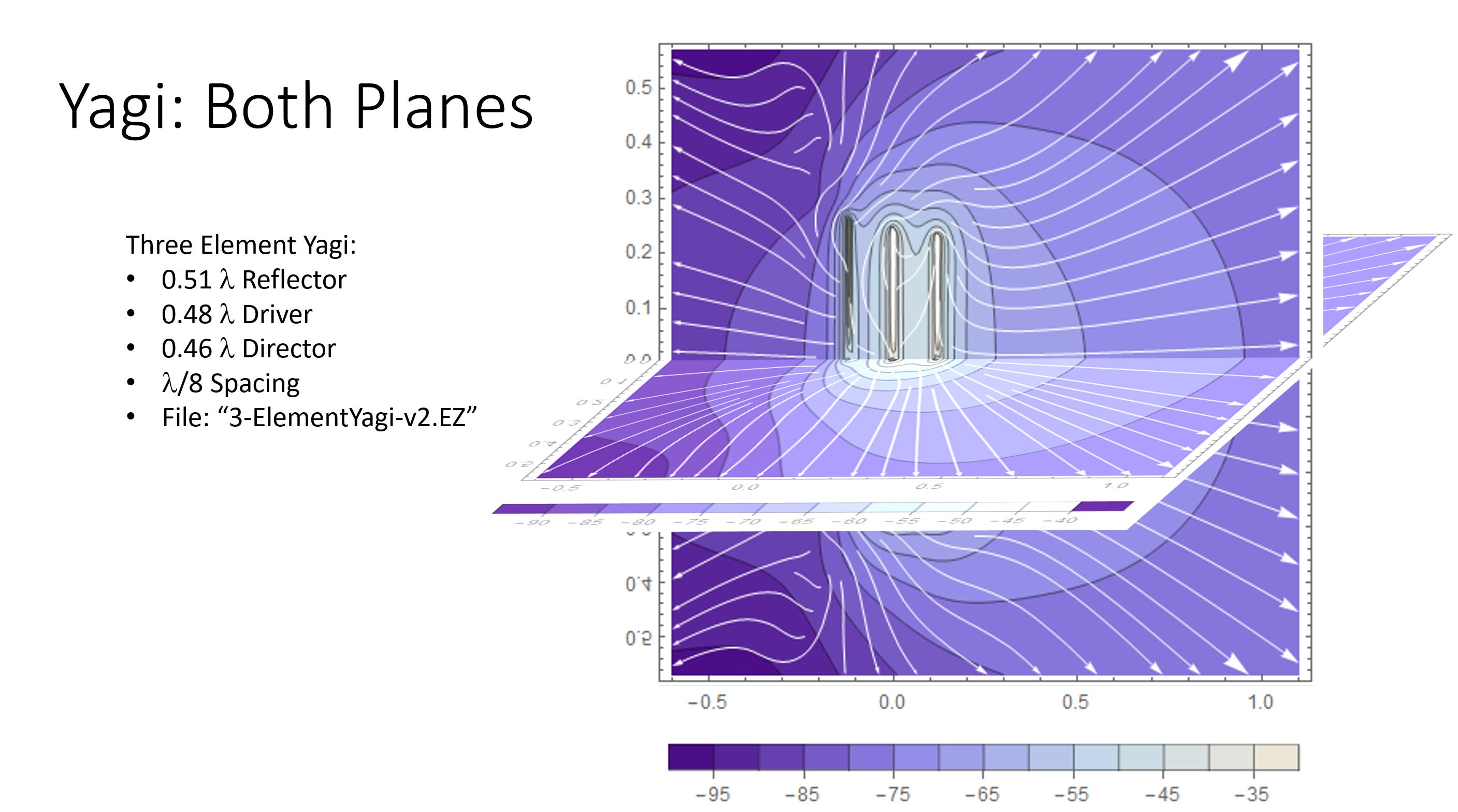
Hans: Yeah, that goes back to my first comment about how valuable it is to have multiple models. I mean, this isn’t a one-size-fits-all solution that’s going to solve all your engineering problems. It is another tool to put in your box, along with your field thinking, along with your transmission line thinking, and... So forth.

What I’ve used it for is looking at energy flow streamlines around ideal dipoles and I used that to design ultra-wideband antennas because I wanted to design antennas that did not support the reactive concentrations of energy that narrow the bandwidth and accommodate themselves to the ideal streamflow lines of energy radiating out.

The Art & Science of Ultrawideband Antennas, 2^nd ed. p. 332.

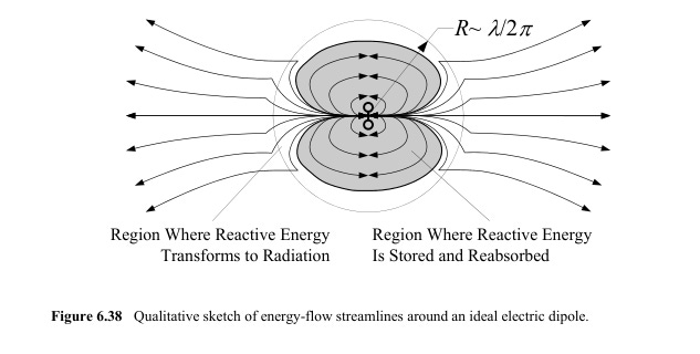
It turns out that gives you a lot of the common shapes that other people had already used, but there were a few in there that were novel, that I was able to invent and ended up doing some of the first commercial ultra-wideband antennas for Time Domain Corporation. It also proved very useful in understanding near fields.

This is probably the application of most interest in the EMC arena. Because when I started doing near-field wireless systems, you need a link law. And Friis’ law assumes everything’s far-field. So by using the energy flow characteristics from small dipole antennas, I ended up figuring out how to do it.

And in fact, I can tell you, if you are trying to certify a Part 15 device to the FCC rules, they assume all antennas are operating in the far field, even when you’re in the far field. So by making a clever selection between electric versus magnetic antennas, you can buy yourself 20 dB or more of extra margin depending on how you conduct the same test according to the officially sanctioned rules. Which is a problem I did not want to call attention to while my livelihood depended on making systems in case they changed them in some way that would make all of our products obsolete.

But paying attention to how near fields work, how you have a balance of energy in the far field, but then as you are close to a source, whether that’s an antenna or a source of interference, you know you can’t count on finding the interference if you use just a magnetic probe or just an electric probe.

You really need to look at both because it could be either.

Question: Is it the streamlines of the Poynting vector or do you need some extra information?

Hans: It’s all in the Poynting vector. The tricky part is taking the field of Poynting vectors and connecting them with streamflow lines. In fact, in the plots that I show, Mathematica, which is what I use to generate them, It wouldn’t give me physically… I wanted streamflow lines where they all started as source. And it would just take random parts out in the side lobe and start something in the middle and track the flow of energy in the side lobe. So I haven’t figured out a good way to do really good valid streamflow lines.

I’ll add that it’s also helpful to keep track of the value of the normalized Lagrangian so you can see where you have balanced energy moving at the speed of light or a concentration of electrostatic or magnetostatic energy from an interference of some kind. Sarkar and Antar have done some wonderful work along these lines.

Benoit: I’m going to take one final question. Oh, he answered your question.

Hans: Up front here?

Benoit: Okay. Well, I’m going to take two final questions then. And then we’ll go.

Question: You mentioned the right-hand rule works for radiated fields? Can RC modeled ESD events have a magnetic sphere that is concentrated a particular point and differ between air discharge versus direct discharge events?

Hans: I don’t know the answer to that. I mean, certainly whenever you have a discharge event and you have something that’s roughly approximating an exponential decay, you’re going to get that kind of behavior where the magnetic field is going to cancel out. In fact, this has been observed in lightning studies, for instance.

Benoit: Thank you. And last question.

Question: Do I understand correctly that this point inductor flow lines applies to the time averaged point inductor field? Time independent. Time independent averaged in the sense that it becomes time independent.

Hans: Yeah, I’m using a couple different kinds of analysis. Like when you take a look at the one interesting thing, and I did this in the philosophical transactions paper on energy, velocity, and reactive fields. The impedance of the exponential decay turns out to be time invariant. Even though the electric and magnetic fields are both decaying, they’re decaying in sync with each other, so you have a constant map of the impedance through this arena. So doing the time domain approach gives you a really good picture of the evolution of a system. But when you start doing things like, you’re taking a look at, this is a time average point.

So there’s other stuff going on that is tough to capture outside of an animation if you want to see it. So yeah, you really have to use both the time-dependent form to get the minor details of how things are behaving, and then the time-average form gives you the big picture.

And the plots that I was showing later on are all showing time-average behavior from sinusoidal sources.

Question: Yes, some time ago I had a publication where I looked at instantaneous fields, of this field, of the back, of the back field, and they look completely different than the time average field. They can, yes. Yes, and do you have any thoughts about physical interpretation of those projections?

Hans: Well, I do think that along with Maxwell, Heaviside, and Poynting, I do think that it reflects a real flow of energy that can be stored in empty space around our electromagnetic systems. And by tracking that flow, you can gain insights that are of use to practical problems.

Question: That’s what I tried to do, but unfortunately I couldn’t find a good interpretation of what I can calculate.

Benoit: Thank you. Maybe it’s a good discussion to continue during the break and during the rest of the day. I want to thank again the speaker Hans for a great talk and great answer to all these questions and thank the audience. Thank you everyone. Thank you. And I have a coin for you.

---

That’s all for now. Remember always to keep calm, and make physics great again.

More soon,

Hans

Follow Online:

You may follow me online in other places as well:

• Telegram: 𝔸𝕖𝕥𝕙𝕖𝕣𝕔𝕫𝕒𝕣’𝕤 𝔸𝕖𝕥𝕙𝕖𝕣𝕤𝕥𝕣𝕖𝕒𝕞

• Gab: @aetherczar

• Twitter: @aetherczar

• Amazon: Hans G. Schantz

• ResearchGate

• Google Scholar

• ORCID